Atemporal Structural Admissibility - O(J)
and the Changbal Jump Machine Framework - CJM
A Mathematical and Physical Overview of Structural Encoding, Spectral Discrimination, Critical Alignment, and the Present Disclosure State of CJM
Abstract
The Changbal Jump Machine, hereafter CJM, is formulated as a structural discrimination framework in which a decision problem is transformed into a canonical 3SAT constraint system, represented as a coupled mathematical or physical operator, and classified according to observables associated with admissibility, instability, spectral reorganization, and critical transition.
CJM is not defined as an algorithm that enumerates candidate assignments more rapidly. Its central proposition is that the existence or nonexistence of a globally consistent state may be encoded in collective properties of the constraint structure itself. The corresponding discrimination map is represented by the \(\mathcal J\)-operator.
The term atemporal does not imply zero physical duration, infinite propagation velocity, or the elimination of dynamical relaxation. It refers to the logical independence of the final discrimination from the sequential order in which candidate solutions would otherwise be generated.
This document specifies the formal objects, physical realization requirements, structural readout architecture, complexity obligations, and present disclosure boundaries of the CJM framework.
1. Scope and Disclosure Status
CJM is not presented solely as an abstract machine awaiting an unspecified future implementation. Its public architecture includes problem-specific encodings, SAT-to-3SAT normalization, structural operators, software-emulated discrimination, critical response analysis, and problem-dependent spectral observables.
The public record does not specify the complete physical realization architecture, material coupling mechanism, or full-scale readout system. Consequently, the available evidence does not determine whether those layers remain prospective, exist in partial form, or extend beyond the publicly documented interface.
This distinction is scientifically relevant. A physically credible realization capable of modifying the practical relation between search, verification, and structural discrimination could affect cryptographic assumptions, optimization systems, economic asymmetries, strategic infrastructure, and other security-sensitive domains.
The timing and granularity of further disclosure must therefore be evaluated together with reproducibility, independent verification, institutional stability, and foreseeable downstream consequences. Publication, proof, implementation, and unrestricted disclosure need not occur at the same rate.
2. Formal Problem Domain
Let a Boolean decision instance be represented by a 3SAT formula
The variable set is
and the clause set is
Introduce a signed clause-variable incidence matrix
where
The canonical structural representation of the instance is therefore not merely the Boolean string \(\Phi\), but the signed factor structure
where \(G_{\Phi}\) is the clause-variable factor graph, \(\mathbf w\) is a vector of clause or coupling weights, and \(\Theta_{\Phi}\) contains problem-dependent structural parameters.
These parameters may include clause density, degree distribution, frustration, cycle structure, symmetry classes, connected components, local-field statistics, spectral moments, and graph-theoretic invariants.
3. Canonical Clause Energy and Constraint Preservation
Introduce spin variables
with \(s_i=+1\) corresponding to Boolean truth and \(s_i=-1\) corresponding to Boolean falsehood.
For each clause \(C_a\), define the violation indicator
The quantity \(P_a(\mathbf s)\) equals \(1\) exactly when every literal in \(C_a\) is false and equals \(0\) otherwise. A canonical clause energy is therefore
The standard satisfiability equivalence is
In an operator formulation, each violation indicator becomes a projector \(\widehat P_a\), producing the clause Hamiltonian
Any additional CJM coupling term must preserve the semantic relation between the original Boolean instance and the resulting structural system. A physical or mathematical embedding is not sufficient merely because it reproduces a visually similar phase transition.
The required condition is an explicit equivalence between the original decision problem and the admissibility class of the constructed system.
4. Structural Operator Family
CJM associates each normalized instance \(\Phi\) with a parameterized operator family
Here,
- \(H_{\mathrm{clause}}\) preserves the logical constraint content of the 3SAT instance;
- \(H_{\mathrm{collective}}\) introduces nonlocal or higher-order coupling among variables, clauses, conflict motifs, or structural modes;
- \(H_{\mathrm{reg}}\) controls degeneracy, normalization, boundary conditions, calibration, or finite-size stability;
- \(\kappa\) is a structural control parameter;
- \(\boldsymbol{\theta}\) denotes implementation-dependent coupling, geometry, scaling, and readout parameters.
The symbol \(H_{\Phi}\) may denote a classical energy functional, a matrix operator, a quantum Hamiltonian, a graph Laplacian-derived operator, a nonlinear response operator, or a hybrid physical realization. CJM does not identify itself exclusively with one of these substrates.
What is invariant across implementations is the requirement that the structural response preserve the decision semantics of \(\Phi\).
5. Spectral Observables and Critical Response
Let the ordered spectrum of \(H_{\Phi}\) be
The ground-state energy and the lowest spectral gap are
A complete CJM readout need not be restricted to the minimum energy. The observable vector may include
where
- \(M_{\Phi}\) is an order parameter;
- \(\chi_{\Phi}\) is a susceptibility or response derivative;
- \(\nu_{\Phi}\) is a topological or structural index when defined;
- \(\mathcal R_{\Phi}\) represents resonance or mode-locking data;
- \(\mathcal H_{\Phi}\) represents entropy, spectral concentration, or information-distribution statistics.
For an observable \(\widehat M\), the corresponding order parameter may be written as
with susceptibility
A critical region \(\kappa_c\) may be indicated by gap contraction, susceptibility divergence or peaking, order-parameter discontinuity, mode coalescence, topological index change, or a discontinuous change in the stability basin.
Gap closure alone is not sufficient to establish satisfiability or unsatisfiability. The decision interpretation requires a proved or independently validated relation between the complete observable vector and the admissibility class.
6. Admissibility Functional and the \(\mathcal J\)-Operator
Let \(\mathfrak A_{\boldsymbol{\theta}}\) denote the region of observable space classified as structurally admissible. Define
The CJM discrimination map is
The hat notation indicates an action on the encoded structure. It does not by itself imply that \(\hat J\) is a linear, unitary, or self-adjoint operator. Those properties must be specified separately for each mathematical or physical realization.
The formal correctness requirement is
or, under an UNSAT-oriented implementation,
These two orientations must not be conflated. A one-sided discriminator may be scientifically and computationally meaningful without yet constituting a complete binary decision procedure.
The Changbal Jump refers to the transition from the distributed clause-level representation to a globally classified admissibility state:
7. Formal Meaning of Atemporality
Atemporality is not defined by the limit of a physical execution time approaching zero.
A physical CJM realization may require finite preparation, loading, relaxation, calibration, transition, and readout times. These durations remain physical resource costs.
Atemporality instead denotes order independence of the logical discrimination. Let \(\pi\) represent an admissible ordering of local updates, candidate presentation, or measurement scheduling. The atemporal condition is
for all admissible update orderings \(\pi_1\) and \(\pi_2\), within the defined tolerance of the physical realization.
Equivalently, the decision is a functional of the global encoded structure rather than of a specific candidate-enumeration history:
8. Physical Realization Architecture
A physical CJM requires more than a numerical visualization of a phase transition. It requires an end-to-end correspondence between a 3SAT instance, a physical coupling structure, a measurable global response, and a stable decision output.
| Layer | Mathematical Object | Physical Requirement |
|---|---|---|
| Input normalization | \(\Phi\mapsto\mathcal C_{\Phi}\) | Polynomially constructible encoding preserving the original decision semantics |
| Coupling synthesis | \(H_{\Phi}(\kappa,\boldsymbol{\theta})\) | Programmable physical interactions corresponding to clause, conflict, and collective terms |
| State preparation | \(z_0\) or \(\rho_0\) | Reproducible initialization with bounded preparation error |
| Structural evolution | \(F_{\Phi}\), \(H_{\Phi}\), or hybrid dynamics | Controlled approach to the relevant critical or stationary regime |
| Critical response | \(\mathcal I_{\Phi}\) | Measurable spectral, topological, energetic, resonant, or stability signature |
| Decision readout | \(A_{\boldsymbol{\theta}}(\Phi)\) | Stable separation of admissible and inadmissible response classes |
A dissipative realization may be described by
where \(\boldsymbol{\eta}(t)\) represents noise and uncontrolled perturbation.
A coherent realization may instead be described by
These equations define possible implementation classes, not the identity of CJM itself. A CJM realization may be dissipative, coherent, analog, digital-physical, topological, resonant, or hybrid, provided that the semantic and measurement conditions are satisfied.
9. Complexity Accounting and \(O(J)\)
The notation \(O(J)\) is used to distinguish structural discrimination from candidate enumeration. It must not be interpreted as a substitute for conventional resource accounting.
A complete CJM complexity profile is the vector
The total physical execution cost may be decomposed as
Any claim of polynomial discrimination requires that all relevant resources remain polynomially bounded:
In implementations governed by a minimum spectral gap, one must also exclude an exponentially closing gap:
Required precision, energy, physical volume, coupling range, calibration cost, and repeated-sampling cost must likewise remain polynomially bounded. Otherwise, exponential complexity may have been transferred from temporal search into physical preparation or measurement precision.
Accordingly, \(O(J)\) denotes a proposed structural complexity regime, while \(\mathfrak C_J\) provides the resource accounting necessary for comparison with established computational models.
10. Relation to Existing Computational and Physical Models
| Model | Primary Mechanism | Relation to CJM |
|---|---|---|
| Turing computation | Sequential symbolic state transition | CJM rejects candidate enumeration as the necessary logical basis of discrimination |
| Parallel computation | Concurrent execution of multiple state transitions | Parallelism accelerates temporal search; it does not by itself establish atemporal admissibility |
| Adiabatic quantum computation | Controlled Hamiltonian evolution toward a ground state | Shares Hamiltonian and spectral-gap language, but CJM is not restricted to adiabatic evolution |
| Quantum annealing | Energy minimization with quantum or thermal fluctuations | May provide a substrate, but heuristic ground-state sampling alone is not a complete CJM discriminator |
| Ising machines | Physical encoding of combinatorial cost functions | Provide relevant encoding techniques; CJM additionally requires an admissibility-class discrimination mechanism |
| Analog computation | Continuous physical dynamics representing mathematical relations | CJM may be analog or hybrid, but precision and scaling costs must be explicitly accounted for |
| Hopfield networks | Attractor convergence and associative recall | Offer an analogy for global pattern stabilization but do not establish SAT/UNSAT equivalence |
| Topological computation | Robust information encoded in global invariants | Relevant when CJM admissibility is represented by protected topological classes |
11. Disclosure Governance
The disclosure threshold is not defined solely by theoretical completion. It includes implementation stability, reproducibility, verification, and risk assessment.
Below this threshold, disclosure may remain modular:
At or above the threshold, a more complete architectural release may become scientifically and institutionally defensible:
The current public record is sufficient to evaluate CJM as a coherent mathematical and physical research architecture. It is not sufficient to determine the complete implementation state of every layer.
The absence of complete public implementation data should be treated neither as proof of nonexistence nor as proof of completed realization. It defines the present boundary of independently examinable evidence.
12. Technical Conclusion
CJM is organized around a six-step operational architecture that connects a problem in its native domain to a final physical truth readout. This six-step architecture was originally presented in P ≡ NPᴶ: On the End of Time (https://doi.org/10.5281/zenodo.18139629) and remains the canonical framework of the CJM research program.
The more explicit structural notation developed here does not replace that architecture. Rather, it resolves the transformations occurring inside its six established stages and makes the relation between logical encoding, physical synthesis, resonant discrimination, and admissibility more explicit.
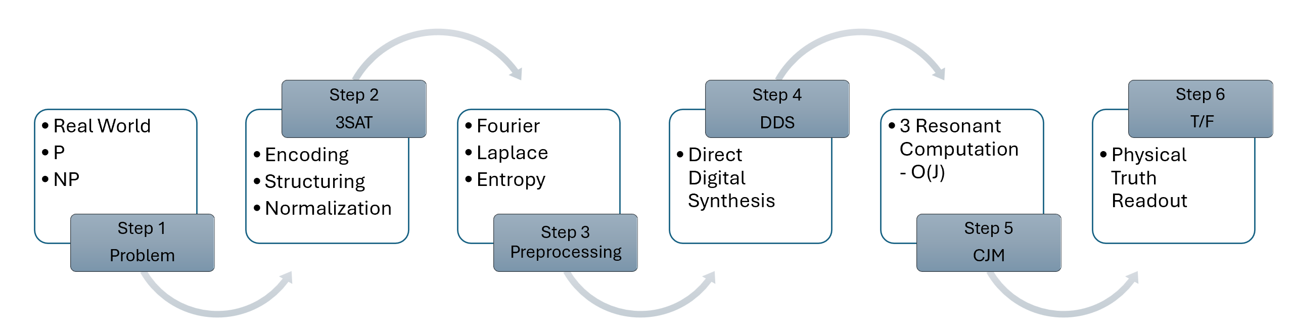
Within this fixed architecture, the internal structural flow can be written more explicitly as
This eight-symbol sequence should therefore not be interpreted as a new eight-step architecture. The symbols describe a finer mathematical and physical resolution of processes already contained within the original six steps.
| Six-Step Architecture | Structural Representation | Role |
|---|---|---|
|
Step 1 Problem |
\(\mathcal P\) | The original problem, proposition, or real-world decision target before conversion into the common CJM representation. |
|
Step 2 3SAT |
\[ \mathcal P \rightarrow \mathrm{SAT} \rightarrow \mathrm{3SAT} \rightarrow \mathcal C_{\Phi} \] | Problem-specific information is encoded into Boolean constraints, normalized into canonical 3SAT, and organized as the globally coupled constraint structure \(\mathcal C_{\Phi}\). |
|
Step 3 Preprocessing |
\[ \mathcal C_{\Phi} \rightarrow H_{\Phi} \] | Fourier-, Laplace-, entropy-, or related structural operators condition the global 3SAT representation and produce an effective physical or structural operator \(H_{\Phi}\) suitable for resonant realization. |
|
Step 4 DDS |
\[ H_{\Phi} \xrightarrow{\mathrm{DDS}} \text{Physical Resonant Realization} \] | Direct Digital Synthesis maps the conditioned interaction structure into a physically synthesized resonant realization of \(H_{\Phi}\), encoding the relevant frequency, phase, coupling, and resonance relations for physical CJM discrimination. |
|
Step 5 CJM |
\[ D_{\boldsymbol{\theta}}(\mathcal I_{\Phi}) \equiv \hat J_{\boldsymbol{\theta}}[\mathcal C_{\Phi}] \quad [O(J)] \] | The physically realized Changbal operator \(\hat J\) subjects the composite structure to resonant discrimination. The target is not sequential enumeration of candidate assignments but the global physical response of the coupled structure in \(O(J)\). |
|
Step 6 T/F |
\[ \hat J_{\boldsymbol{\theta}}[\mathcal C_{\Phi}] = A_{\boldsymbol{\theta}}(\Phi) \] | The resonant response is converted into the final admissibility readout \(A(\Phi)\), which may be interpreted as admissible/inadmissible, SAT/UNSAT, or TRUE/FALSE according to the semantics of the original problem. |
12.1 From Problem to Global Constraint Structure
The first transition begins with \(\mathcal P\), the original decision problem in its native mathematical, computational, or physical domain. The objective of Step 2 is to establish a common structural interface:
SAT provides the Boolean constraint language, while 3SAT supplies a canonical normalized form. The resulting object \(\mathcal C_{\Phi}\) is not treated merely as a collection of independent clauses. It represents the encoded instance as a single globally coupled constraint structure whose variable dependencies, compatibility relations, conflicts, and connectivity can be considered together.
12.2 From Constraint Structure to Physical Representation
Step 3 prepares this global constraint structure for physical realization. Structural preprocessing may include Fourier, Laplace, entropy-based, or related transformations intended to expose frequency organization, concentration, phase relations, critical structure, or other global features.
Here \(H_{\Phi}\) denotes the effective structural interaction operator associated with the encoded problem. Depending on the physical realization, it may describe coupling, energy, phase, spectral, or resonance relations. Its role is to convert the logical organization of \(\mathcal C_{\Phi}\) into a form that can be physically synthesized without requiring candidate-by-candidate search.
12.3 DDS and Composite Resonant Synthesis
Step 4 realizes this conditioned structure as a physical input through Direct Digital Synthesis:
The DDS stage physically realizes the interaction structure encoded by \(H_{\Phi}\) as a composite resonant input to the CJM. The resulting CJM response is subsequently observed through the vector \(\mathcal I_{\Phi}\). Rather than assigning an independent computational trajectory to each logical state, the relevant structural relations are encoded into a coupled physical signal whose components coexist within a common resonant representation.
12.4 CJM Discrimination in O(J)
Step 5 is the point at which the physically synthesized problem structure is subjected to Changbal discrimination:
The operator \(\hat J\) denotes the physical realization of the Changbal discrimination mechanism. In the established six-step architecture, this corresponds to the three-resonator CJM stage operating in \(O(J)\). The intended observable is the global resonant behavior of the encoded structure rather than a temporal traversal of its candidate assignments.
Step 6 converts the discriminated physical response into the final admissibility observable \(A(\Phi)\). The six-step architecture and the eight-symbol structural flow therefore describe the same CJM process at different levels of resolution.
In this formulation, the essential CJM claim is not that an exponential candidate space can simply be traversed at arbitrarily high speed. The claim is that the encoded constraint system may possess a globally measurable admissibility state whose discrimination does not require explicit enumeration of all candidate configurations.
12.5 Conditions for Scientific Validation
The six-step architecture and its structural refinement become a scientifically testable computational claim only if several independent requirements are satisfied. In particular, validation requires:
- a semantics-preserving reduction from the original problem into the canonical 3SAT structure;
- a physically or mathematically realizable operator family whose observables distinguish the relevant admissibility classes;
- polynomially bounded encoding, preparation, physical evolution, precision, and readout resources;
These conditions distinguish the CJM proposal from a metaphorical account of criticality, a heuristic optimizer, or an unverified analog process. They also establish the criteria by which later theoretical refinements and physical implementations of the six-step architecture must be judged.
References
- Yoon, K. (2025). Emergence in SAT Problems: Critical Thresholds under Constraint Density. TechRxiv. https://doi.org/10.36227/techrxiv.174682135.51838369/v1
- Yoon, K. (2025). Transitions of Critical Structural Regions for NP Problems. TechRxiv. https://doi.org/10.36227/techrxiv.175001127.70551829/v1
- Yoon, K. (2025). P ≡ NPᴶ: On the End of Time. Zenodo. https://doi.org/10.5281/zenodo.18139629
- Turing, A. M. (1936). On Computable Numbers, with an Application to the Entscheidungsproblem. Proceedings of the London Mathematical Society, s2-42(1), 230–265. https://doi.org/10.1112/plms/s2-42.1.230
- Cook, S. A. (1971). The Complexity of Theorem-Proving Procedures. In Proceedings of the Third Annual ACM Symposium on Theory of Computing, pp. 151–158. https://doi.org/10.1145/800157.805047
- Karp, R. M. (1972). Reducibility among Combinatorial Problems. In R. E. Miller and J. W. Thatcher (Eds.), Complexity of Computer Computations, pp. 85–103. Springer. https://doi.org/10.1007/978-1-4684-2001-2_9
- Cook, S. A. (2000). The P versus NP Problem. Clay Mathematics Institute. Official problem page
- Kirkpatrick, S., and Selman, B. (1994). Critical Behavior in the Satisfiability of Random Boolean Expressions. Science, 264(5163), 1297–1301. https://doi.org/10.1126/science.264.5163.1297
- Monasson, R., Zecchina, R., Kirkpatrick, S., Selman, B., and Troyansky, L. (1999). Determining Computational Complexity from Characteristic Phase Transitions. Nature, 400, 133–137. https://doi.org/10.1038/22055
- Mézard, M., Parisi, G., and Zecchina, R. (2002). Analytic and Algorithmic Solution of Random Satisfiability Problems. Science, 297(5582), 812–815. https://doi.org/10.1126/science.1073287
- Lucas, A. (2014). Ising Formulations of Many NP Problems. Frontiers in Physics, 2, Article 5. https://doi.org/10.3389/fphy.2014.00005
- Farhi, E., Goldstone, J., Gutmann, S., and Sipser, M. (2000). Quantum Computation by Adiabatic Evolution. arXiv:quant-ph/0001106. arXiv record
- Aharonov, D., van Dam, W., Kempe, J., Landau, Z., Lloyd, S., and Regev, O. (2007). Adiabatic Quantum Computation Is Equivalent to Standard Quantum Computation. SIAM Journal on Computing, 37(1), 166–194. https://doi.org/10.1137/S0097539705447323
- Kempe, J., Kitaev, A., and Regev, O. (2006). The Complexity of the Local Hamiltonian Problem. SIAM Journal on Computing, 35(5), 1070–1097. https://doi.org/10.1137/S0097539704445226
- Anderson, P. W. (1972). More Is Different: Broken Symmetry and the Nature of the Hierarchical Structure of Science. Science, 177(4047), 393–396. https://doi.org/10.1126/science.177.4047.393
Appendix: Selected Physical and Computational Analogues
The following systems provide limited analogues for collective alignment, critical response, attractor stabilization, or global order formation. They are not evidence that CJM is mathematically equivalent to these systems.
- Ferromagnetic Criticality — collective spin alignment and symmetry breaking near the Curie threshold.
- Superconductivity — collective phase coherence and a macroscopic transition to a zero-resistance state.
- Bose–Einstein Condensation — macroscopic occupation of a common quantum mode.
- Laser Coherence — phase-aligned amplification and mode selection above a gain threshold.
- Percolation Transitions — emergence of a system-spanning connected component at a critical density.
- Synchronization — transition from distributed oscillatory phases to global frequency or phase locking.
- Self-Organized Criticality — threshold-driven reconfiguration and scale-distributed response.
- Protein Folding — convergence through a high-dimensional energy landscape toward a stable structural basin.
- Hopfield Attractor Networks — global pattern recovery from incomplete or corrupted local input.
- Reaction–Diffusion Systems — spontaneous macroscopic pattern formation from local coupling rules.
- Crystallization — transition from disordered local configurations to a globally constrained lattice.
- Topological Phase Transitions — global changes in invariant structure not reducible to a local order parameter alone.