Sep 15, 2025
We frame NP problems not as targets for mere statistical cleaning but for transformative reinterpretation prior to solving. To illustrate this idea, we present three representative preprocessing methods: Fourier-Guided Preprocessing (FGP), Laplace-Guided Preprocessing (LGP), and Entropy-Guided Preprocessing (EGP). These methods reshape instance structure through a signalization–domain adjustment–discrete remapping pipeline, exposing sharp shifts in solvability.
On Subset Sum, all three alter the phase-transition profile; on SAT and 2-Coloring on 3-uniform hypergraphs, continuous operators (FGP/LGP) may disrupt combinatorial consistency, whereas EGP preserves discreteness while shifting the location or widening the width of the transition region. These findings support a simple principle: transformation precedes computation. Preprocessing is thus recast as a guided lens that clarifies solvability transitions before any learning or search.
Our contributions are: (i) a cross-domain comparison of the three methods under a unified perspective; (ii) evidence that, when combinatorial semantics must be preserved, EGP is a reliable baseline; and (iii) a modular formalization of FGP/LGP/EGP with a common interface for transplantation into preprocessing stages beyond NP tasks. We provide runnable code and experiment settings for reproducibility, and outline how learning-based components can be layered on these clarified inputs. Beyond NP problems, we envision this approach being extended to diverse complex systems, including physical signal processing, biological networks, and social systems.
Keywords: NP problems, preprocessing, Fourier transform, Laplace transform, Entropy analysis, structural analysis, AI intervention, problem solvability, phase transitions, entropy-guided preprocessing
Solvability in NP problems can change nonlinearly as structural factors (e.g., constraint density and variable interactions) vary, indicating that instance structure, not just algorithms, is decisive for tractability.
Conventional preprocessing (imputation, outlier handling, normalization) targets statistical hygiene rather than structural insight, whereas SAT-specific preprocessing has been extensively studied in the literature . In contrast, physical–mathematical transforms offer lenses for structural reinterpretation prior to solving.
We therefore introduce three reusable modules—Fourier-Guided Preprocessing (FGP), Laplace-Guided Preprocessing (LGP), and Entropy-Guided Preprocessing (EGP). Each module independently instantiates the same three-stage internal template—signalization, domain adjustment, and discrete remapping—without implying any sequential composition across modules. Depending on the task/domain, a single module may be applied selectively, with parallel evaluation used only for comparison. We position FGP/LGP/EGP as leading exemplars of a broader, open-ended family of domain-informed preprocessing methods; the shared template is designed to accommodate future modules. All three share a common interface to support transplantation into preprocessing stages beyond NP tasks (e.g., signal processing, graph learning, reinforcement learning).
This work builds directly on our prior studies of critical structural
transitions under constraint density , and connects to prior
research that has used entropy and solution density to characterize SAT
structure . At the same time, our
definition of entropy draws on foundational concepts from information
theory ,
shifting the focus upstream to the preprocessing phase as a bridge
between raw instances and downstream methods. Building on these
foundations, we adopt the terminology of Changbal concepts introduced in
our earlier studies. Specifically, we refer to the sharp collapse point
as the Changbal Point, the narrow surrounding interval as the Changbal
Region, and the corresponding trajectory as the Changbal Curve. These
terms emphasize that the phenomena observed here are not merely
algorithmic artifacts but structural markers of emergent
solvability.
Definition (Changbal Concepts).
Our hypothesis is simple: transformation precedes computation.
By restructuring the instance to expose and stabilize transition
signals—while preserving combinatorial semantics—we obtain inputs that
are measurably easier to analyze or learn from. We evaluate the effect
of FGP/LGP/EGP on Subset Sum, SAT, and 2-Coloring.
This section introduces three independent, reusable preprocessing modules—Fourier-Guided Preprocessing (FGP) , Laplace-Guided Preprocessing (LGP) , and Entropy-Guided Preprocessing (EGP) —that restructure NP instances prior to any learning or search. These modules do not solve the problems directly; rather, they re-express latent structure into more tractable forms and make transition signals measurable. The trio is not exhaustive: they serve as leading exemplars of an open-ended family of domain-informed preprocessing methods. Each module implements the same three-stage internal template (signalization \(\rightarrow\) domain adjustment \(\rightarrow\) discrete remapping) through a common interface, but no sequential composition across modules is implied. Depending on the task/domain, a single module may be applied selectively, with parallel evaluation used only for comparison. The reference stubs for Python, Java, and C are not provided merely as ancillary code samples but as a general-purpose, modular infrastructure designed for immediate adoption across both academic and industrial domains. In practice, Python remains the dominant environment for rapid prototyping and AI research; Java underpins enterprise-scale frameworks in finance, telecommunications, and security; and C continues to serve as the backbone for high-performance computing (HPC), embedded systems, and kernel-level optimizations.
By releasing harmonized stubs in these three foundational languages, this work ensures that researchers and practitioners can seamlessly integrate the proposed preprocessing modules into diverse pipelines—from AI model training and optimization workflows to industrial software architectures—without the burden of rewriting or adapting code across environments. The cross-language modularization thus elevates the contribution of this study from a theoretical framework to a platform-level enabler of practical applications and interdisciplinary transfer.
Reference stubs for Python, Java, and C are available at GitHub (Python/Java/C stubs) (accessed Sep 15, 2025).
| Method | Domain | Purpose and Effect |
|---|---|---|
| (Fourier- | ||
| Guided) | Frequency | Filters dominant structural frequencies to remove repetitive or noisy patterns, enhancing clarity of solvable cores. |
| (Laplace- | ||
| Guided) | ||
| Graph | Smooths irregularities using Laplacian eigenvalues to highlight global and essential structural patterns. | |
| (Entropy- | ||
| Guided) | ||
| Profiling | Detects entropy-based irregularities by modeling distributional shifts, revealing hidden structural transitions. |
FGP maps an instance to a 1D/ND signal (signalization), moves it to the frequency domain, applies a guided band mask, and inverts back, followed by discrete remapping that preserves combinatorial semantics (e.g., clause length, \(k\)-uniformity). This separates dominant repetitions (lower bands) from high-frequency irregularities, yielding inputs that are more stable for downstream analysis or learning.
\[\mathrm{FGP}_{\alpha}(x)\;=\;\mathcal{T}\!\left(\,\mathcal{F}^{-1}\!\big(\,\Phi_{\alpha}\!\left(\mathcal{F}(\mathrm{signalize}(x))\right)\big)\right),\] where \(\mathcal{F}\)/\(\mathcal{F}^{-1}\) denote (discrete) Fourier transform and its inverse, \(\Phi_{\alpha}\) is a guided mask operator parameterized by band/strength, and \(\mathcal{T}\) is a discrete remapping rule designed to preserve combinatorial constraints. In practice we use the DFT: \[S_k=\sum_{n=0}^{N-1} s_n\,e^{-2\pi i kn/N},\qquad s_n=\frac{1}{N}\sum_{k=0}^{N-1} S_k\,e^{2\pi i kn/N}.\]
Analyzing constraint sequences or structural graphs in the frequency domain isolates repeated motifs and suppresses disruptive fluctuations. Proper masking can shift or stabilize transition signals without breaking discrete semantics; overly aggressive smoothing, however, risks semantic violations, hence the need for guards.
import numpy as np

def fgp_transform(instance, signalize, discretize, guard,
                  band=("low", 0, 10), mask_type="soft",
                  threshold=None, seed=42):
    # 1) map instance -> numeric signal
    s = signalize(instance)                 # domain-specific
    # 2) forward DFT
    S = np.fft.fft(s)
    # 3) guided band mask in frequency domain
    S_t = apply_guided_mask(S, band=band, mode=mask_type)
    # 4) inverse + discrete remapping
    s_inv = np.fft.ifft(S_t).real
    inst_p = discretize(s_inv, threshold)
    # 5) semantics guard (fail/rollback if violated)
    if not guard(inst_p):
        raise ValueError("Combinatorial semantics violated.")
    return inst_p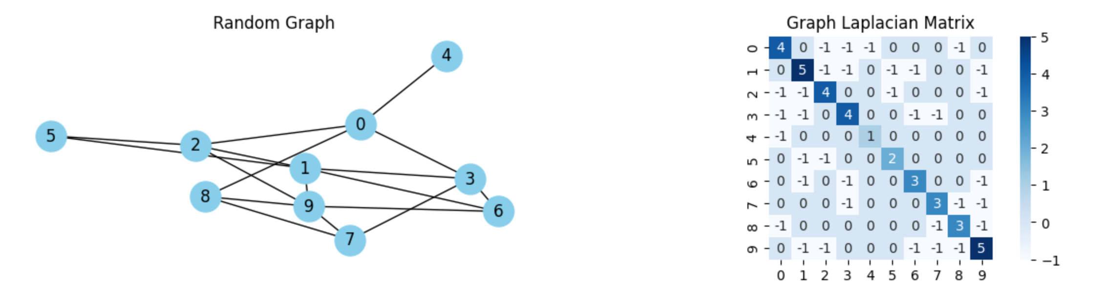
LGP leverages the (graph) Laplacian spectrum to detect and smooth structural irregularities in an instance’s graph representation. By attenuating high-frequency components while preserving combinatorial semantics at remapping time, LGP clarifies global structure without implying any sequential composition with other modules.
\[L = D - A \quad , \qquad \tilde{x} \;=\; U\, g_{\beta}(\Lambda)\, U^{\top} x,\] where \(D\) and \(A\) are the degree and adjacency matrices, \(L = U \Lambda U^{\top}\) is the eigendecomposition, and \(g_{\beta}(\cdot)\) is a low-pass spectral filter (e.g., heat kernel \(g_{\beta}(\lambda)=e^{-\beta \lambda}\)). An equivalent iterative view is diffusion: \(x_{t+1} = x_t - \alpha L x_t\).
Low-frequency eigenvectors capture global structure; high-frequency components often reflect noise or local irregularities. Projecting onto a low-frequency subspace (or applying diffusion) yields a smoothed representation that highlights essential patterns, after which discrete remapping restores a valid combinatorial instance.
import networkx as nx
import numpy as np

def lgp_transform(G, discretize, guard, k=3, use_heat_kernel=False, beta=0.3):
    # 1) Build Laplacian (combinatorial; normalized variants are also possible)
    L = nx.laplacian_matrix(G).astype(float).toarray()
    # 2) Eigendecomposition (symmetric => eigh)
    eigvals, eigvecs = np.linalg.eigh(L)

    if use_heat_kernel:
        # Heat kernel smoothing: U exp(-beta Lambda) U^T x
        # Here we illustrate node-wise features x as the all-ones vector
        x = np.ones((L.shape[0], 1))
        H = eigvecs @ np.diag(np.exp(-beta * eigvals)) @ eigvecs.T
        x_smooth = H @ x
        G_smooth = discretize(x_smooth, params={})
    else:
        # Low-frequency reconstruction using the smallest-k eigenvectors
        U_k = eigvecs[:, :k]
        P = U_k @ U_k.T  # projector onto low-frequency subspace
        # Example: project adjacency rows/columns (domain-specific choices apply)
        A = nx.to_numpy_array(G)
        A_smooth = P @ A @ P
        G_smooth = discretize(A_smooth, params={})

    # 3) Semantics guard: must preserve combinatorial constraints
    if not guard(G_smooth):
        raise ValueError("Combinatorial semantics violated by LGP output.")
    return G_smooth
EGP interprets the diversity and organization of constraint states through entropy—a measure of disorder that can signal phase transitions or emergent structure.
\[S = -k \sum_{i} p_i \log p_i\]
Here, \(S\) is the entropy of the system, \(k\) is the Boltzmann constant (set to \(1\) for normalization), and \(p_i\) represents the probability of each structural state.
By computing the entropy of constraint distributions, one can evaluate whether the system is in a high-disorder (chaotic) or low-disorder (emergent structure) state. This informs when and where to apply structural reorganization for better AI effectiveness.
import numpy as np

# Example distribution of structural states
p = np.array([0.1, 0.3, 0.4, 0.2])

# Compute entropy (Boltzmann constant k = 1)
S = -np.sum(p * np.log(p))Before introducing any transformation techniques, we first establish the foundational structure used throughout this study: the basic subset structure. This structure represents a preprocessed form of the original NP instance, designed to extract latent signals without introducing bias .
Even in its raw form, this subset structure begins to expose underlying patterns, laying the groundwork for analyzing solvability transitions .
Without applying any external transformation (Fourier, Laplace, or Entropy methods), the subset structure itself already exhibits signs of nonlinear transitions. Specifically, we observe sharp shifts in solvability outcomes—an early manifestation of the Changbal Point and Changbal Region.
This implies that structural properties alone—not yet guided or amplified—already encode emergent features. Thus, understanding the basic subset is essential for isolating and amplifying these nonlinearities in the next stages.
While the raw subset structure reveals early emergence, it lacks precision, consistency, and control. Three key reasons necessitate structural transformation:
Uncaptured subtle patterns: Some high-impact patterns are buried in noise or irregular distributions.
High variance in transition boundaries: The emergence threshold fluctuates unpredictably across problem instances.
Difficulty in guiding AI intervention (J-Factor): Without structured preprocessing, the application of AI models cannot reliably identify critical transition areas.
These limitations call for applying principled preprocessing methods that reshape the subset structure to more clearly reveal and amplify the Changbal Region. The next chapter presents three such transformation techniques—Fourier, Laplace, and entropy-guided methods—and demonstrates how each affects solvability.
In this chapter, we apply each of the three preprocessing methods—Fourier, Laplace, and Entropy modeling—to the subset structure introduced in Chapter 3. The transformation leverages classical signal-processing techniques: for instance, bilinear mappings between continuous- and discrete-time domains underpin Fourier/Laplace–based recharacterization . Meanwhile, the Entropy modeling draws on Jaynes’ information-theoretic framework, where entropy serves as a lens to interpret structural order . We analyze how each transformation reshapes the base structure and prepares data for AI learning.
Each subsection explores one of the three methods in detail, including:
the transformation process applied to the subset structure,
the resulting changes in the emergence curve and structural properties,
and the preparation of transformed data for downstream AI applications.
This structured exploration illustrates how preprocessing techniques not only reveal hidden solvability transitions but also generate standardized, learnable representations for AI-based intervention models.
To investigate latent regularities within the subset structure, we apply the Fourier transform directly to the numerical array of each instance in the Subset Sum problem. This method maps structural sequences into the frequency domain, allowing us to detect dominant periodic patterns and filter out high-frequency noise that may obscure solvability signals.
We treat each input array as a one-dimensional time-domain signal, where the value of each element reflects its contribution to the total sum. By applying the Discrete Fourier Transform (DFT), we convert this signal into the frequency domain, isolate the low-frequency components, and reconstruct a smoothed version of the original array using the inverse transform.
Let \(x = \{x_0, x_1, \dots, x_{n-1}\}\) be the input array. The DFT is computed as: \[X_k = \sum_{j=0}^{n-1} x_j \cdot e^{-2\pi i k j / n}, \quad \text{for } k = 0, 1, \dots, n-1.\] By retaining only the first few coefficients in \(X_k\), we eliminate high-frequency components and reduce structural oscillation. The resulting smoothed array is then clipped to remain within the valid range \([1, \text{element\_max}]\) and reinterpreted as a new instance of the problem.
Figure 6 presents the empirical comparison between the raw and Fourier-transformed input arrays in terms of success rate over increasing target sums. The transformed curve shows a clearer sigmoidal shape and an earlier (leftward) transition point, indicating a more stable structural progression.
| Metric | Raw | Fourier | \(\Delta\) (F–R) |
|---|---|---|---|
| Transition location \(r^\ast\) | 420.00 | 362.22 | \(-57.78\) |
| \(T_{0.1}\) (10% success) | 472.00 | 436.92 | \(-35.08\) |
| \(T_{0.9}\) (90% success) | 343.64 | 306.15 | \(-37.48\) |
| Width \(w = |T_{0.9}-T_{0.1}|\) | 128.36 | 130.77 | \(+2.41\) |
| Slope \(k \approx 2\ln 9 / w\) | 0.03423 | 0.03360 | \(-0.00063\) |
| Metric | Raw | Fourier | \(\Delta\) (F–R) |
|---|---|---|---|
| Mean success over \(T\) (AUC\(\sim\)) | 0.513 | 0.435 | \(-0.079\) |
| Total variation (TV) of curve | 1.020 | 1.000 | \(-0.020\) |
| Uncertainty area \(\sum p(1-p)\) | 1.501 | 1.571 | \(+0.070\) |
| Curve \(L_2\) gap \(Q\) | – | – | 0.559 |
Quantitatively, Table 2 shows that the 50% transition point \(r^\ast\) shifts from \(420.00\) (Raw) to \(362.22\) (Fourier), i.e., \(\Delta r^\ast = -57.78\). The 10%/90% crossing points also move earlier (\(T_{0.1}\): \(472.00 \rightarrow 436.92\), \(\Delta = -35.08\); \(T_{0.9}\): \(343.64 \rightarrow 306.15\), \(\Delta = -37.48\)), while the width is similar (\(w=128.36\) vs. \(130.77\), \(\Delta w=+2.41\)) and the implied slope changes only marginally (\(k=0.03423\) vs. \(0.03360\), \(\Delta k=-0.00063\)). Auxiliary metrics in Table 3 are consistent with this picture: the mean success over targets decreases (AUC\(\sim\): \(0.513 \rightarrow 0.435\)), total variation slightly reduces (\(1.020 \rightarrow 1.000\)), the uncertainty area increases modestly (\(1.501 \rightarrow 1.571\)), and the \(L_2\) curve gap is sizable (\(Q=0.559\)).
Taken together, the earlier \(r^\ast\), largely unchanged width, and reduced total variation indicate that Fourier preprocessing yields structurally smoother instances whose transition signal emerges sooner and with lower volatility. Although the average success across targets decreases, the clearer sigmoidal profile and distinct curve gap suggest that solvability signals are more consistently expressed, which can benefit learning-based methods that rely on stable structure–response relationships.
We evaluate two Laplacian variants applied to Subset Sum arrays prior to solving: (i) a discrete second-derivative Laplacian mask that highlights local structural changes, and (ii) iterative Laplacian smoothing (local averaging, \(k{=}3\)) that reduces short-range fluctuations. Unlike Fourier filtering that targets harmonics, Laplacian operators emphasize large-scale structure via local differencing/averaging.
Using the kernel \([1,-2,1]\) on array \(A\) and adding the scaled response back (\(A+\alpha\,\Delta A\), \(\alpha{=}0.5\)) mildly sharpens edges: \[(\Delta A)[i]=A[i{+}1]-2A[i]+A[i{-}1].\] Figure 7 shows a slight leftward shift and mild sharpening. Quantitatively (Table 4): \(r^\ast\) moves from \(420.00\) to \(392.94\) (\(\Delta=-27.06\)), width decreases (\(-3.36\)), slope increases slightly (\(+0.00093\)), mean success drops by \(0.019\), TV reduces by \(0.020\), uncertainty area decreases (\(-0.083\)), and the curve gap is \(Q{=}0.213\).
| Metric | Raw | Laplace | \(\Delta\) (L–R) |
|---|---|---|---|
| Transition location \(r^\ast\) | 420.00 | 392.94 | \(-27.06\) |
| \(T_{0.1}\) (10% success) | 472.00 | 465.00 | \(-7.00\) |
| \(T_{0.9}\) (90% success) | 343.64 | 340.00 | \(-3.64\) |
| Width \(w = |T_{0.9}-T_{0.1}|\) | 128.36 | 125.00 | \(-3.36\) |
| Slope \(k \approx 2\ln 9 / w\) | 0.03423 | 0.03516 | \(+0.00093\) |
| Mean success over \(T\) (AUC\(\sim\)) | 0.513 | 0.494 | \(-0.019\) |
| Total variation (TV) | 1.020 | 1.000 | \(-0.020\) |
| Uncertainty area \(\sum p(1-p)\) | 1.501 | 1.418 | \(-0.083\) |
| Curve \(L_2\) gap \(Q\) | – | – | 0.213 |
Local averaging (applied \(k{=}3\) times) replaces each element by the mean of its neighbors, \[A_{\text{smooth}}[i]=\frac{A[i{-}1]+A[i]+A[i{+}1]}{3},\] with boundary handling. Figure 8 exhibits a clearer sigmoid with an earlier and wider transition. Table 5: \(r^\ast\) shifts to \(374.12\) (\(\Delta=-45.88\)), width increases (\(+10.57\)), slope decreases (\(-0.00260\)), mean success drops by \(0.054\), TV is slightly higher (\(+0.040\)), uncertainty area is roughly unchanged (\(+0.007\)), and \(Q{=}0.409\).
| Metric | Raw | Laplace | \(\Delta\) (L–R) |
|---|---|---|---|
| Transition location \(r^\ast\) | 420.00 | 374.12 | \(-45.88\) |
| \(T_{0.1}\) (10% success) | 472.00 | 451.43 | \(-20.57\) |
| \(T_{0.9}\) (90% success) | 343.64 | 312.50 | \(-31.14\) |
| Width \(w = |T_{0.9}-T_{0.1}|\) | 128.36 | 138.93 | \(+10.57\) |
| Slope \(k \approx 2\ln 9 / w\) | 0.03423 | 0.03163 | \(-0.00260\) |
| Mean success over \(T\) (AUC\(\sim\)) | 0.513 | 0.459 | \(-0.054\) |
| Total variation (TV) | 1.020 | 1.060 | \(+0.040\) |
| Uncertainty area \(\sum p(1-p)\) | 1.501 | 1.508 | \(+0.007\) |
| Curve \(L_2\) gap \(Q\) | – | – | 0.409 |
Both variants bring the transition earlier (leftward \(r^\ast\)). The mask is a light-touch operator that slightly sharpens the profile (narrower \(w\), larger \(k\)) while reducing variability (TV, uncertainty area). Smoothing is a stronger intervention: it advances \(r^\ast\) more and widens the critical zone (larger \(w\), smaller \(k\)), making the decline more gradual—useful when robust, low-variance structure is desired.
Masked arrays surface edge-like cues (useful for detectors of local irregularity), while smoothed arrays provide low-variance contexts for learning global patterns. In both cases, features such as low-order spectral energies, Laplacian response statistics, and transition-position proxies (\(r^\ast, T_{0.1}, T_{0.9}\)) can supervise signal-aware GNNs or sequence models.
We evaluate two entropy-guided transformations that restructure Subset Sum arrays prior to solving. Unlike frequency/spectral operators (FGP/LGP), EGP modifies value distributions to probe how dispersion and cumulative energy shape the solvability transition.
Given an array \(A\), we reweight entries by an entropy-like score \[A'_i \;=\; -\log\!\Big(\tfrac{A_i}{\sum_j A_j}\Big),\] which suppresses dominant magnitudes and highlights dispersion. Empirically (Fig. 9), this yields curves that deviate from Raw with generally lower success rates but clearer expression of distributional effects.
| Metric | Raw | ||
| (Entropy) | \(\Delta\) (E–R) | ||
| Transition location \(r^\ast\) | 420.00 | 395.56 | \(-24.44\) |
| \(T_{0.1}\) (10% success) | 472.00 | 469.09 | \(-2.91\) |
| \(T_{0.9}\) (90% success) | 343.64 | 333.33 | \(-10.30\) |
| Width \(w = |T_{0.9}-T_{0.1}|\) | 128.36 | 135.76 | \(+7.39\) |
| Slope \(k \approx 2\ln 9 / w\) | 0.03423 | 0.03237 | \(-0.00186\) |
| Mean success over \(T\) (AUC\(\sim\)) | 0.513 | 0.487 | \(-0.026\) |
| Total variation (TV) of curve | 1.020 | 1.020 | \(0.000\) |
| Uncertainty area \(\sum p(1-p)\) | 1.501 | 1.375 | \(-0.126\) |
| Curve \(L_2\) gap \(Q\) | – | – | 0.295 |
Sort \(A\) by magnitude and retain the smallest prefix whose cumulative sum reaches a ratio \(\alpha\) of the total: \[\sum_{i=1}^{k} A_{(i)} \;\le\; \alpha \!\cdot\! \sum_{j=1}^{n} A_j \quad (\alpha{=}0.7).\] This truncation (Fig. 10) reduces instance size and often depresses success, exposing failure-side structure at the cost of combinatorial richness.
| Metric | Raw | ||
| (Entropy) | \(\Delta\) (E–R) | ||
| Transition location \(r^\ast\) | 420.00 | 303.33 | \(-116.67\) |
| \(T_{0.1}\) (10% success) | 472.00 | 357.33 | \(-114.67\) |
| \(T_{0.9}\) (90% success) | 343.64 | 260.00 | \(-83.64\) |
| Width \(w = |T_{0.9}-T_{0.1}|\) | 128.36 | 97.33 | \(-31.03\) |
| Slope \(k \approx 2\ln 9 / w\) | 0.03423 | 0.04515 | \(+0.01091\) |
| Mean success over \(T\) (AUC\(\sim\)) | 0.513 | 0.280 | \(-0.234\) |
| Total variation (TV) of curve | 1.020 | 1.000 | \(-0.020\) |
| Uncertainty area \(\sum p(1-p)\) | 1.501 | 1.029 | \(-0.472\) |
| Curve \(L_2\) gap \(Q\) | – | – | 1.604 |
EGP does not aim to “boost” success; it reveals how dispersion (entropy) and low-energy truncation modulate the transition. Reweighting pulls the distribution toward uniformity, while cutoff foregrounds failure regimes. Together, they provide complementary views of the solution landscape for downstream models.
Low-order histogram features (e.g., normalized counts, spectral entropy), cutoff ratio \(\alpha\), and transition proxies (\(T_{0.1}, T_{0.9}, r^\ast\)) serve as compact features for signal-aware GNNs/Transformers.
Tables 6 and 7 report Raw vs. EGP in the same format as the Fourier/Laplace tables.
Entropy reweighting advances the transition modestly and slightly widens the critical region, whereas energy cutoff drives a large leftward shift while narrowing the region; both reduce AUC\(\sim\), more strongly for cutoff.
In this section, we extend the core hypothesis of this study—that structural preprocessing acts as a lens for reinterpreting the inherent difficulty of NP problems—by applying the three preprocessing methods (Fourier, Laplace, and Entropy) from Chapter 4 to new problem domains. Specifically, we consider two canonical NP-complete problems: the Boolean satisfiability problem (3-SAT), a paradigmatic testbed for phase-transition phenomena , and the 2-Coloring problem on uniform hypergraphs, which exemplifies combinatorial coloring hardness and threshold effects. We analyze the effects of these methods on the satisfiability and average solving time for 3-SAT and 2-Coloring problems, aiming to explore structural changes in their phase transitions and further solidify our main thesis.
We validate the effectiveness of our preprocessing techniques on 3-SAT problem instances with \(n=60\) variables. By varying the constraint density \(r\) from \(2.0\) to \(6.1\), we measure the satisfiability ratio and average solving time at each point to analyze how preprocessing affects the problem’s difficulty and structure.
The change in the satisfiability ratio according to the preprocessing methods is presented in Figure 11.
Raw: The raw, unprocessed problem instances show a typical phase transition phenomenon where the satisfiability ratio drops sharply from 1 to 0 at approximately \(r \approx 4.2\). This point represents the critical threshold where the hardest instances of the SAT problem are concentrated.
EGP: The instances preprocessed with the Entropy method show a curve similar to the raw data, but the critical threshold is subtly shifted to the right, to approximately \(r \approx 4.5\). This suggests that the entropy-based preprocessing has softened the problem’s structure, extending the region where solutions can be found even under a higher constraint density.
FGP and LGP: Both of these preprocessing techniques show a sharp drop in the satisfiability ratio to near 0 starting around \(r \approx 2.5\). This indicates that the structural integrity of the problems was severely damaged during preprocessing, leaving a solution space that is virtually non-existent.
Next, we analyze the effect of each preprocessing method on the average solving time, as shown in Figure 12.
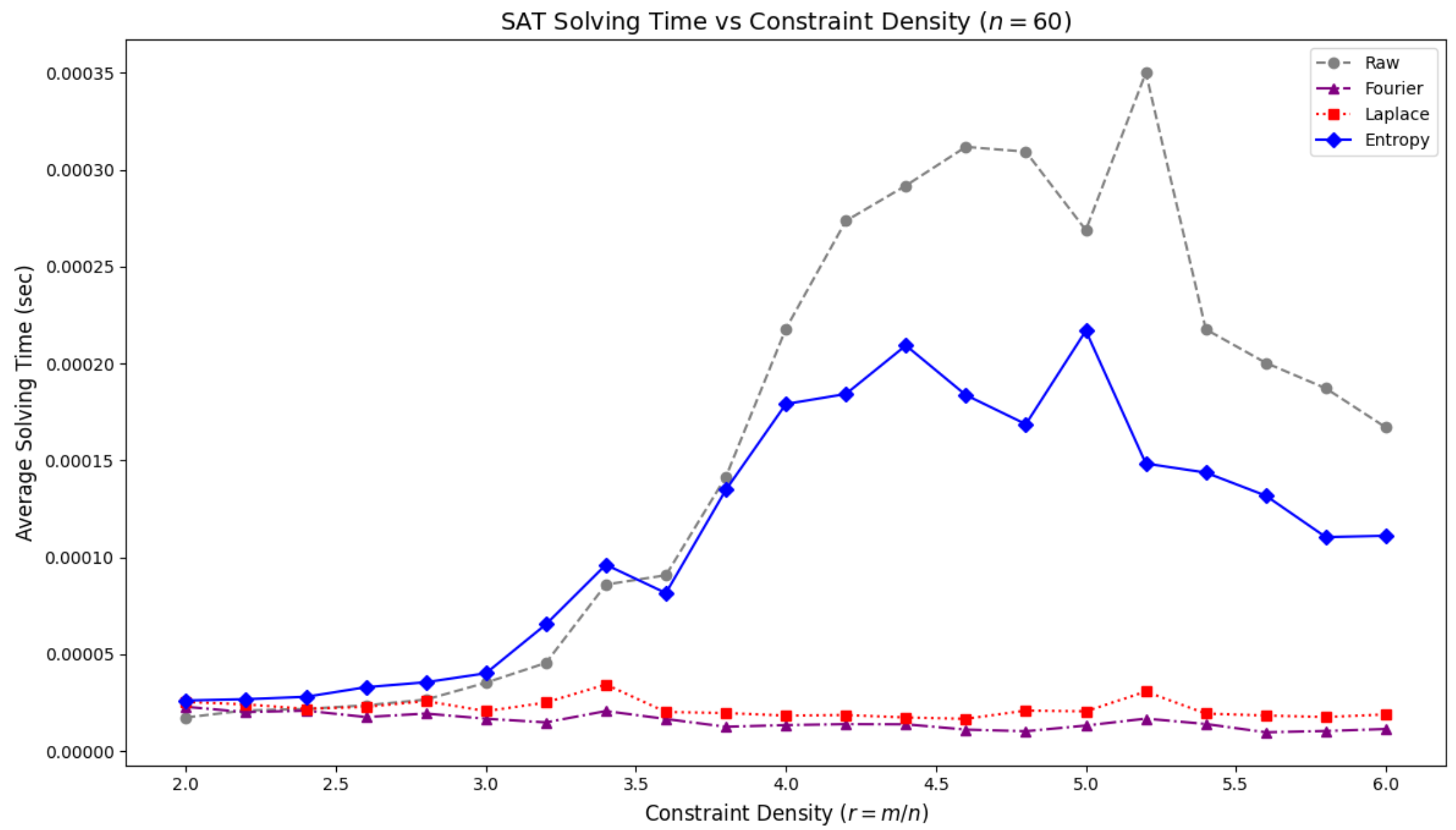
Raw: The raw instances show a peak in average solving time near the phase transition point of \(r \approx 4.5\). This peak corresponds to the region where the solver performs the most extensive search to find a solution.
EGP: When Entropy preprocessing is applied, the peak in solving time shifts slightly to a higher density of \(r \approx 4.7\), and its height is significantly reduced compared to the raw data. This suggests that preprocessing has both mitigated the difficulty of the hardest problems and dispersed the phase transition region more broadly across a wider range of constraint densities.
FGP and LGP: Both of these methods resulted in very short solving times, regardless of the value of \(r\). This aligns with the satisfiability ratio analysis, as the solver quickly declares failure for problems that are rendered effectively unsolvable.
In this section, we apply the preprocessing techniques to the 2-Colorability problem of a 3-uniform hypergraph to validate their effects. We fixed the number of vertices at \(n=12\) and varied the constraint density \(r\) from \(0.5\) to \(5.1\), measuring the proportion of 2-colorable instances.
The change in the 2-Coloring success rate according to the preprocessing methods is presented in Figure 13.
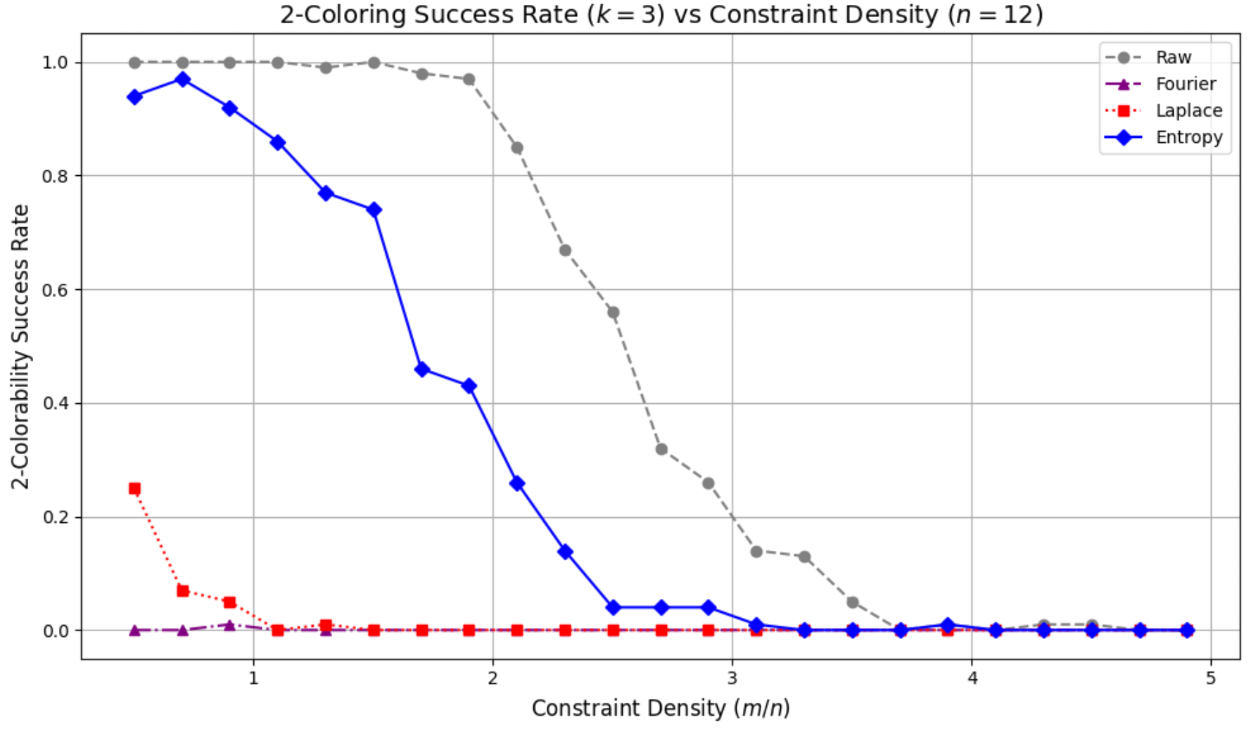
Raw: The raw, unprocessed hypergraph instances show a sharp phase transition where the success rate drops significantly around \(r \approx 2.0\). This point serves as the critical threshold for the 2-Coloring problem.
EGP: The instances processed with the Entropy method show a phase transition that shifts to the right, occurring at approximately \(r \approx 2.5\). This observation suggests that entropy-based preprocessing can soften the problem’s structure, thereby expanding the region of solvability even under increased constraint density.
FGP and LGP: Both of these methods show a success rate that remains near 0 from very low \(r\) values. This indicates that the preprocessing severely corrupted the combinatorial structure of the problem, destroying the possibility of a valid coloring.
The series of experiments on the Subset Sum, SAT, and 2-Coloring problems conclusively demonstrates that preprocessing is not merely a tool for performance optimization but a lens for reinterpreting the inherent structure of a problem.
In the Subset Sum problem, which has a continuous, number-based structure, all three preprocessing techniques (Fourier, Laplace, and Entropy) proved effective in altering the phase transition region. In contrast, for the combinatorial and discrete problems of SAT and 2-Coloring, the continuous operations of Fourier and Laplace preprocessing failed catastrophically by destroying the problem’s underlying logical structure. The Entropy method, however, which operates on a statistical concept (entropy) that preserves the discrete nature of the variables, showed consistent positive effects.
The entropy-based Entropy preprocessing consistently demonstrated its effectiveness across all tested NP problems. By controlling the inherent disorder of the problem, it consistently shifted the phase transition point to the right or otherwise mitigated difficulty, regardless of the problem’s specific domain (numeric or combinatorial). This suggests that the Entropy approach is a robust and universally applicable tool for reinterpreting the structure of diverse NP problems.
In conclusion, this research proves that the choice of a preprocessing technique can fundamentally alter the solvability and difficulty of a problem. This finding highlights the critical need for a strategic approach to preprocessing, viewing it as a ’structural reinterpretation’ of the problem, which is essential for designing effective future AI-based solution strategies.
This chapter synthesizes the findings from previous sections to examine the broader impact of structural preprocessing on problem solvability. Rather than focusing on individual methods, we aim to provide a unified perspective that highlights the recurring patterns and underlying principles observed across multiple problem domains. These principles resonate with the insights offered by Lucas, who showed that many NP-complete problems—including Karp’s classic 21—can be systematically mapped to Ising models, suggesting a shared structural lens across diverse NP-hard domains . These insights help pave the way toward a structural understanding of emergence in NP-complete problems.
This section analyzes how the three proposed preprocessing methods—Fourier-based decomposition, Laplace-based smoothing, and Entropy filtering—affect the structural composition of NP-complete problems. Experimental results suggest that these techniques do not simply reduce solving time, but induce meaningful reconfigurations in the constraint landscape, aligning with recent trends in applying graph neural networks (GNNs) to SAT solving tasks, where structural transformations directly influence model performance . The observed changes in satisfiability ratio and solver performance indicate that solvability transitions are closely linked to the structural state of the problem instance. Accordingly, structural preprocessing can be considered a catalyst that exposes latent regions of tractability.
Although the current study does not directly utilize machine learning models, the clarity and regularity achieved through structural preprocessing suggest promising directions for future integration. The emergence of smoother transition curves and identifiable solvability regions may enhance the performance of learning-based algorithms such as Graph Neural Networks (GNNs) and Deep Reinforcement Learning (DRL). Recent studies show how GNNs can learn structural features to predict SAT satisfiability and guide solver strategies , while DRL has demonstrated effectiveness in neural combinatorial optimization by learning powerful heuristics for NP-hard problems . These structural improvements can serve as inputs or conditioning factors, potentially simplifying the model’s learning task. This section outlines possible quantitative indicators (e.g., entropy reduction, clause overlap patterns) that can guide the integration of AI models in future work.
Synthesizing observations across SAT, 3-uniform hypergraph 2-Coloring and subset problems, this section proposes a unifying interpretation: emergent solvability arises from transitions in the problem’s structural domain rather than from changes in algorithmic heuristics. The consistent appearance of narrow, critical zones—termed “Changbal Regions”—across multiple NP-complete domains (including SAT, Subset Sum, and 3-uniform hypergraph 2-Coloring) suggests the presence of a generalized structural phenomenon, echoing earlier statistical-physics analyses of constraint satisfaction landscapes . These regions, characterized by nonlinear shifts in success rates and solving time, align with the broader view that phase transitions provide a structural lens on computational complexity . Such regions can be revealed or expanded through preprocessing, opening the door to a structural theory of solvability in NP problems, where transformation precedes computation.
While the preceding preprocessing experiments revealed shifts in curves and transition widths, the more important purpose of this study is to convert these results into a dataset for AI training—with explicit attention to failure segments where solvability collapses. From each preprocessing output, we extract the following indicators: (1) the critical threshold \(r^\ast\), (2) the transition width \(\Delta r\), (3) the slope at the transition midpoint, (4) success rates at selected levels (e.g., 0.1, 0.5, 0.9), and (5) entropy and variance of the outcome distribution. In addition, we record failure-aware descriptors, including (6) the number and span of low-success regions, (7) the entropy gradient within those regions, (8) a taxonomy of failure patterns (abrupt vs. gradual), and (9) hypothesized structural causes inferred from the transformed instance. All values are stored with the instance ID, problem type, and preprocessing method in a structured format (CSV/JSON).
Why emphasize failures? In learning systems, hard negatives shape the decision boundary, counteracting class imbalance and preventing overfitting to “easy” successes. Failure-centric features improve calibration (probability accuracy), enhance robustness under distribution shift, and provide contrastive signal that makes structural patterns more learnable by representation learners. Consequently, these data serve as input features for Graph Neural Networks (GNNs) and Deep Reinforcement Learning (DRL), enabling models to focus capacity where it matters most—on the ambiguous and intractable regions—rather than merely amplifying already solvable cases. Even if preprocessing alone does not yield immediate solver gains, the induced shifts together with failure-aware uncertainty metrics open a new feature space that is particularly suitable for downstream AI training.
def extract_data(I, M, include_failures=True, seed=42, levels=[0.1, 0.5, 0.9]):
    InitRandomSeed(seed)

    # curves (before / after)
    c0 = ComputeSolvabilityCurve(I)
    I1 = ApplyPreprocessing(I, M)
    c1 = ComputeSolvabilityCurve(I1)

    # transition features (after)
    r_star = FindCriticalThreshold(c1)
    d_r    = MeasureTransitionWidth(c1)
    slope  = ComputeMidpointSlope(c1)
    succ   = EvaluateSuccessRates(c1, levels)
    ent    = CalculateEntropy(c1)
    sfeat  = ExtractStructuralFeatures(I1)

    # optional failure analytics (after)
    fails=fent=fpat=fcause=None
    if include_failures:
        fails  = IdentifyFailureRegions(c1)
        fent   = CalculateFailureEntropyGradient(c1, fails)
        fpat   = ClassifyFailurePatterns(c1, fails)
        fcause = EstimateFailureCauses(I1, c1, fails)

    # impact (before vs after)
    impact = CompareBeforeAfter(c0, c1, r_star, d_r, slope, succ)

    rec = {
        "instance": GetInstanceId(I),
        "problem_type": GetProblemType(I),
        "method": GetMethodId(M),
        "seed": seed,
        "r_star": r_star, "delta_r": d_r, "slope": slope,
        "success": succ, "entropy": ent,
        "structural_features": sfeat,
        "impact": impact,
        "fail_regions": fails, "fail_entropy_grad": fent,
        "fail_patterns": fpat, "fail_causes": fcause
    }
    SaveRecord(rec, format="CSV/JSON")
    return rec
Closing Remark. This study has demonstrated how transformative preprocessing—instantiated via Fourier, Laplace, and Entropy modules—can reshape the structural composition of NP-complete problems, and—more importantly—how the resulting curves can be extracted as datasets for downstream AI applications. Although preprocessing alone may not guarantee immediate solver gains, the induced shifts and uncertainty metrics open a new feature space that is highly learnable by AI models. These concrete findings establish a reproducible basis for structural analysis of solvability transitions.
In this sense, the present paper should be regarded as an entry point. Future research will leverage the extracted datasets to train Graph Neural Networks (GNNs) and Deep Reinforcement Learning (DRL), with the goal of reviving previously intractable regions and turning downward collapse into upward transformation. Rather than merely analyzing solvability curves, the next stage will actively reshape solvability landscapes—demonstrating how AI can move NP-hard instances toward P-like behavior. In other words, the trajectory shifts from experimentally observing emergent transitions to deliberately inducing them, opening a new chapter in the study of emergent solvability in NP-complete problems.
9
A. Biere, M. Järvisalo and B. Kiesl, “Preprocessing in SAT
Solving,” in *Handbook of Satisfiability (Second Edition)*, A.
Biere et al. (eds.), IOS Press, 2021.
Available: Online
Chapter
K. Yoon, “Emergence in SAT Problems: Critical Thresholds under
Constraint Density,” TechRxiv, 2025.
DOI: 10.36227/techrxiv.174682135.51838369/v1
K. Yoon, “Transitions of Critical Structural Regions for NP
Problems,” TechRxiv, 2025.
DOI: 10.36227/techrxiv.175001127.70551829/v1
D. Cohen, “The Impact of Entropy and Solution Density on Selected
Measures in SAT,” *arXiv preprint* (or *PMC*, 2018).
Available: PMC
7513231
J. V. Stone, “Information Theory: A Tutorial Introduction,”
*arXiv preprint*, 2018.
Available: arXiv:1802.05968
A. V. Oppenheim and R. W. Schafer, Discrete-Time Signal
Processing, 3rd edition, Pearson, 2010.
Available (excerpt): PDF
preview via PagePlace
W. H. Hayt, Jr., J. E. Kemmerly, and S. M. Durbin, Engineering
Circuit Analysis, 8th edition, McGraw-Hill, 2012.
Available: PDF
of 8th edition
C. E. Shannon, “A Mathematical Theory of Communication,”
Bell System Technical Journal, vol. 27, no. 3, pp. 379–423, July
1948.
DOI: 10.1002/j.1538-7305.1948.tb01338.x
S. Mertens, “Phase Transition in the Number Partitioning Problem,”
*arXiv preprint*, 1998.
Available: arXiv:cond-mat/9807077
I. P. Gent, “Phase Transitions from Real Computational Problems,”
*Technical Report*, 2003.
Available: CiteSeerX
PDF
A. Venkataraman and A. V. Oppenheim, “Signal Approximation Using the
Bilinear Transform,” *MIT Digital Signal Processing Group Technical
Report*, MIT, 2024.
Available: PDF
available
E. T. Jaynes, “Information Theory and Statistical Mechanics,”
*Physical Review*, vol. 106, no. 4, pp. 620–630, 1957.
DOI: 10.1103/PhysRev.106.620
S. A. Cook, “The Complexity of Theorem-Proving Procedures,”
*Proceedings of the 3rd Annual ACM Symposium on Theory of Computing
(STOC ’71)*, pp. 151–158, 1971.
DOI: 10.1145/800157.805047
R. Monasson, R. Zecchina, S. Kirkpatrick, B. Selman, and L.
Troyansky, “Determining computational complexity from characteristic
‘phase transitions’,” *Nature*, vol. 400, pp. 133–137, 1999.
DOI: 10.1038/22055
A. Lucas, “Ising Formulations of Many NP Problems,” *Frontiers in
Physics*, vol. 2, article 5, 2014.
Available: 10.3389/fphy.2014.00005
I. P. Gent and T. Walsh, “The SAT Phase Transition,” *Proceedings of
the 11th European Conference on Artificial Intelligence (ECAI-94)*, pp.
105–109, 1994.
Available: PDF
via UNSW
J. Tönshoff and M. Grohe, “Learning from Algorithm Feedback: One-Shot
SAT Solver Guidance with GNNs,” *arXiv preprint*, arXiv:2505.16053,
2025.
Available: arXiv:2505.16053
D. Selsam, M. Lamm, B. Bünz, P. Liang, L. de Moura, and D. Dill,
“Learning a SAT Solver from Single-Bit Supervision,” *International
Conference on Learning Representations (ICLR)*, 2019.
Available: arXiv:1802.03685
I. Bello, H. Pham, Q. V. Le, M. Norouzi, and S. Bengio, “Neural
Combinatorial Optimization with Reinforcement Learning,” *arXiv
preprint*, arXiv:1611.09940, 2016.
Available: arXiv:1611.09940
M. Mézard and R. Zecchina, “The random K-satisfiability problem: from
an analytic solution to a new efficient algorithm,” *Physical Review E*,
vol. 66, no. 5, 056126, 2002.
DOI: 10.1103/PhysRevE.66.056126
S. Kirkpatrick and B. Selman, “Critical behavior in the
satisfiability of random Boolean expressions,” *Science*, vol. 264, no.
5163, pp. 1297–1301, 1994.
DOI: 10.1126/science.264.5163.1297
Scientific Python script to analyze the solvability landscape of the Subset Sum problem. This script uses dynamic programming to solve the problem for various target sums (T) and calculates the success rate to identify phase transitions.
import random
import matplotlib.pyplot as plt

# --- 1. Experimental Configuration ---
# A fixed seed is set to ensure that the same pseudo-random sequence is generated
# on every run, guaranteeing the reproducibility of the experimental results.
random.seed(42)

# Define key parameters for the experiment to generate problem instances.
# These parameters directly influence the complexity and solvability landscape.
ARRAY_SIZE = 20          # N: The number of elements in each problem instance array.
ELEMENT_MAX = 40         # R: The maximum integer value for each element (values are in the range [1, R]).
NUM_TRIALS = 50          # M: The number of random problem instances to test for each target sum.
T_RANGE = range(200, 601, 20)  # T_min to T_max: The range of target sums to be tested (the x-axis of the plot).

# --- 2. Data Collection and Experiment Execution ---
# A list to store the measured success rate for each target sum in T_RANGE.
success_rates = []

# Main experimental loop: iterate through each target sum T in the predefined range.
for T in T_RANGE:
    success_count = 0

    # Inner loop: run the experiment for a fixed number of trials to get a statistically
    # significant success rate for the current target sum T.
    for _ in range(NUM_TRIALS):
        # Generate a random problem instance (an array of integers).
        arr = [random.randint(1, ELEMENT_MAX) for _ in range(ARRAY_SIZE)]

        # Dynamic Programming approach to solve the Subset Sum problem.
        # A set 'dp' is used to efficiently track all possible subset sums that can be formed.
        dp = {0}

        # Iterate through each number in the generated array.
        for num in arr:
            # Create a new set to store the updated reachable sums to avoid
            # modifying the set while iterating over it.
            new_dp = set(dp)
            for prev_sum in dp:
                if prev_sum + num <= T:
                    new_dp.add(prev_sum + num)
            # Update the set of reachable sums for the next iteration.
            dp = new_dp

        # Check if the target sum T is present in the set of reachable sums.
        if T in dp:
            success_count += 1

    # Calculate the success rate (probability of a solution existing) for the current T.
    success_rate = success_count / NUM_TRIALS
    success_rates.append(success_rate)
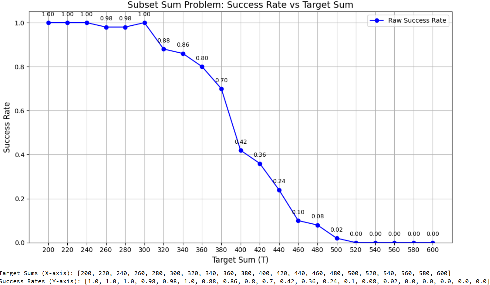
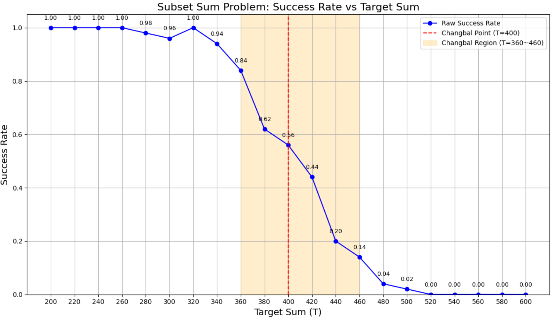
This figure highlights the Changbal Point at T=400 (red dashed line) where solvability sharply drops, and the Changbal Region between T=360–460 (shaded band) where success rates decline steeply. This narrow transition zone illustrates a nonlinear shift from feasible to infeasible instances, showing how computational hardness emerges abruptly rather than gradually.
import random
import matplotlib.pyplot as plt

# --- 1. Experimental Configuration and Reproducibility ---
# A fixed seed is set to ensure that the same pseudo-random sequence is generated
# on every run, guaranteeing the reproducibility of the experimental results.
random.seed(42)

# Define key parameters for generating problem instances.
# These parameters directly influence the complexity and solvability landscape.
ARRAY_SIZE = 20          # N: The number of elements in each problem instance array.
ELEMENT_MAX = 40         # R: The maximum integer value for each element (range: [1, R]).
NUM_TRIALS = 50          # M: The number of random instances to test for each target sum T.
T_RANGE = range(200, 601, 20)  # T_min to T_max: The range of target sums to be tested (x-axis).

# --- 2. Data Collection and Experiment Execution ---
# A list to store the measured success rate for each target sum in T_RANGE.
success_rates = []

# Iterate through the range of target sums to conduct the main experiment.
for T in T_RANGE:
    success_count = 0

    # Run a fixed number of trials to obtain a statistically meaningful success rate.
    for _ in range(NUM_TRIALS):
        # Generate a random problem instance (an array of integers).
        arr = [random.randint(1, ELEMENT_MAX) for _ in range(ARRAY_SIZE)]

        # Dynamic Programming approach to solve the Subset Sum problem.
        # A set 'dp' efficiently tracks all possible subset sums that can be formed.
        dp = {0}

        # Iterate through each number in the generated array.
        for num in arr:
            # Create a new set to store the updated reachable sums to avoid
            # modifying the set while iterating over it.
            next_dp = set(dp)
            for prev_sum in dp:
                # Add the new sum to the set if it does not exceed the target T.
                if prev_sum + num <= T:
                    next_dp.add(prev_sum + num)
            # Update the set for the next iteration.
            dp = next_dp

        # Check if the target sum T is present in the set of reachable sums.
        if T in dp:
            success_count += 1

    # Calculate the success rate (probability of a solution existing) for the current T.
    success_rate = success_count / NUM_TRIALS
    success_rates.append(success_rate)
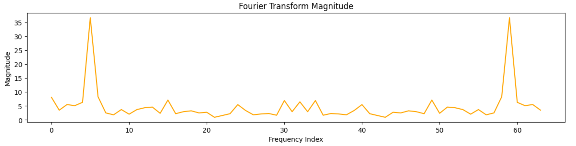
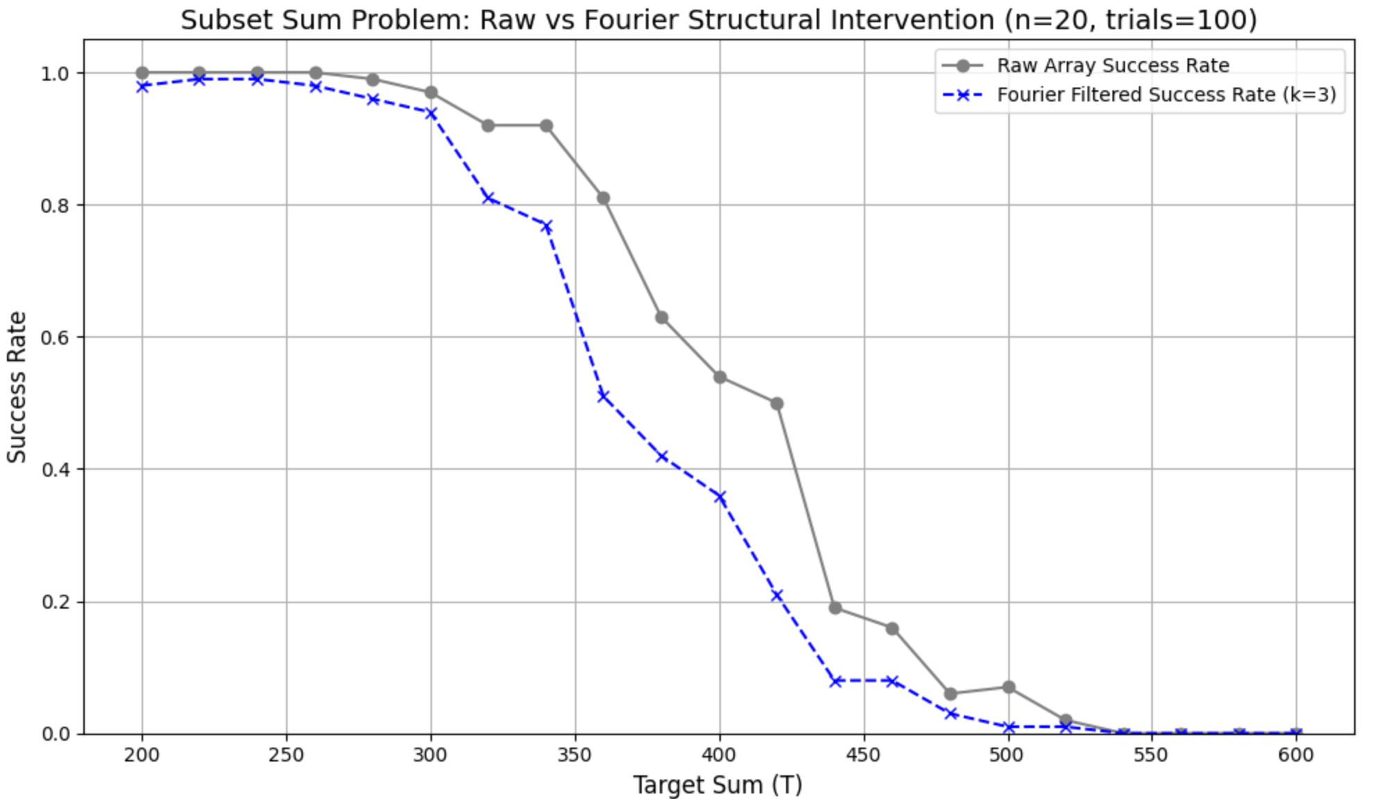
This figure compares the raw success rate (gray line) with the result after applying a Fourier-based structural filter (blue dashed line, k=3). Both curves follow the same overall phase transition, but the Fourier-filtered version shows an earlier and sharper decline, indicating that the structural preprocessing amplifies the emergence of the critical transition. The difference highlights how spectral filtering can shift or reshape the solvability landscape, offering new insight into the Changbal Region.
import numpy as np
import matplotlib.pyplot as plt
from scipy.fft import fft, ifft

# --- Experiment Configuration ---
# Fix the seed for reproducibility
np.random.seed(42)

# Size of the array to be generated randomly
array_size = 20
# Maximum value for elements in the array
element_max = 40
# Number of trials for each target sum (T)
num_trials = 100
# The range of target sums (T) to be tested
T_range = list(range(200, 601, 20))
# Fourier filter parameter
filter_k = 3

# --- 1. Raw Experiment Function ---
def run_raw_experiment():
    """
    Calculates the success rate of the subset sum problem using raw (unfiltered) arrays.
    """
    raw_rates = []
    for T in T_range:
        success_count = 0
        for _ in range(num_trials):
            # Generate a new random array for each trial
            arr = np.random.randint(1, element_max + 1, array_size)

            # Initialize a set for dynamic programming to store possible subset sums
            dp = set()
            dp.add(0)

            # Iterate through all elements of the current array
            for num in arr:
                # Add new sums that do not exceed T
                dp |= {prev_sum + num for prev_sum in dp if prev_sum + num <= T}

            # Check if the target sum T is in the set of possible sums
            if T in dp:
                success_count += 1
        raw_rates.append(success_count / num_trials)
    return np.array(raw_rates)

# --- 2. Fourier-based Structural Intervention Function ---
def run_fourier_experiment():
    """
    Calculates the success rate of the subset sum problem using arrays smoothed by a Fourier filter.
    """
    rates = []
    for T in T_range:
        success_count = 0
        for _ in range(num_trials):
            # Structural smoothing: Generate an array to which Fourier transform can be applied
            arr = np.random.randint(1, element_max + 1, array_size)
            fft_values = fft(arr)

            # Low-pass filtering: Remove high-frequency components to smooth the signal
            filtered_fft = fft_values.copy()
            # Set high-frequency components from filter_k onwards to zero
            filtered_fft[filter_k:] = 0

            # Reconstruct the smoothed array using inverse Fourier transform
            smoothed_arr = np.real(ifft(filtered_fft))

            # Adjust the element range back to [1, element_max] and convert to integer type
            smoothed_arr = np.clip(smoothed_arr, 1, element_max).astype(int)

            # Solve the subset sum problem with the smoothed array
            dp = set()
            dp.add(0)
            for num in smoothed_arr:
                dp |= {prev_sum + num for prev_sum in dp if prev_sum + num <= T}

            # Check if the target sum T is in the set
            if T in dp:
                success_count += 1
        rates.append(success_count / num_trials)
    return np.array(rates)
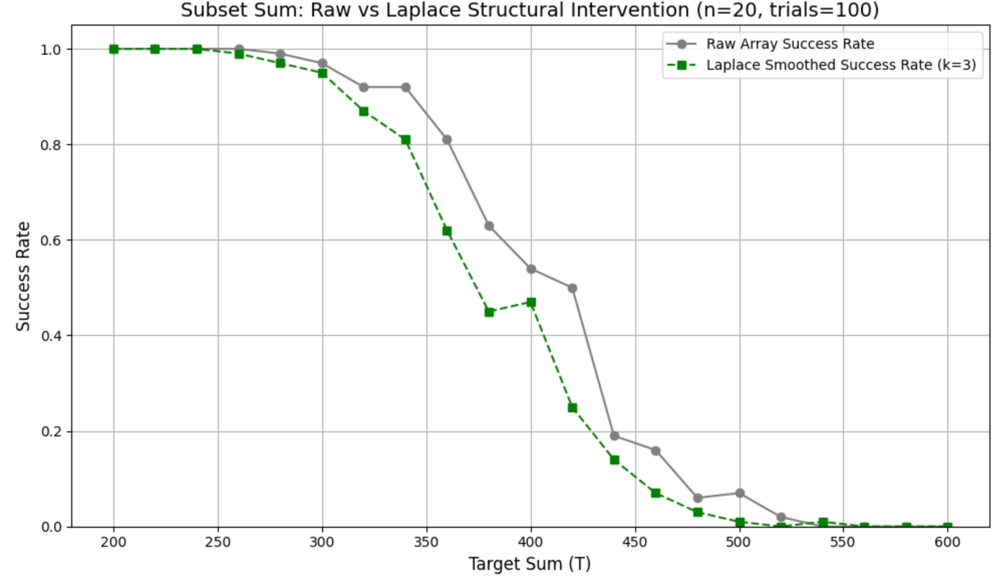
This figure compares the raw success rate (gray line) with the result after applying The Laplacian smoothing (green dashed line, k=3) is compared with the raw success rate (gray line). Unlike Fourier filtering, which shifts the transition globally, the Laplacian mask produces localized, edge-focused modifications. These adjustments slightly alter the slope and fine structure of the decline, particularly near the critical region, while leaving the overall phase transition intact. This demonstrates how Laplacian preprocessing can refine local solvability patterns without fundamentally displacing the Changbal Point.
import numpy as np
import matplotlib.pyplot as plt
from tqdm import tqdm

# --- 1. Experimental Configuration and Reproducibility ---
# A fixed seed is set for both the 'random' and 'numpy' libraries to ensure
# that the same sequence of pseudo-random numbers is generated on every run,
# which is critical for the reproducibility of experimental results.
np.random.seed(42)

# Define key parameters for generating problem instances.
array_size = 20          # N: The number of elements in each problem instance array.
element_max = 40         # R: The maximum integer value for each element (range: [1, R]).
num_trials = 100         # M: The number of random instances to test for each target sum T.
T_range = list(range(200, 601, 20))  # T_min to T_max: The range of target sums to be tested (x-axis).

# Laplace smoothing parameter: The number of times local averaging is applied.
# A higher 'k' value results in a more significant smoothing effect, simulating a
# stronger diffusion of structural properties.
laplace_k = 3

# --- 2. Raw Experiment Function ---
def run_raw_experiment():
    """
    Executes the experiment on the original, unprocessed problem instances.
    It measures the success rate of the Subset Sum problem using a standard
    dynamic programming approach. This serves as the baseline for comparison.
    """
    raw_rates = []
    # Use tqdm for a progress bar, which is useful for long-running experiments.
    for T in tqdm(T_range, desc="Raw"):
        success_count = 0
        for _ in range(num_trials):
            # Generate a random array of integers for the Subset Sum problem.
            arr = np.random.randint(1, element_max + 1, array_size)

            # Dynamic programming approach to find all possible subset sums.
            # A set is used for efficient lookup and insertion.
            dp = {0}
            for num in arr:
                # Efficiently update the set of reachable sums.
                dp |= {s + num for s in dp if s + num <= T}

            # Check if the target sum is in the set of reachable sums.
            if T in dp:
                success_count += 1
        raw_rates.append(success_count / num_trials)
    return np.array(raw_rates)

# --- 3. Laplace Preprocessing Experiment Function ---
def run_laplace_experiment():
    """
    Executes the experiment on problem instances that have been preprocessed
    with Laplace-inspired smoothing. It measures the change in success rate
    due to this structural intervention.
    """
    laplace_rates = []
    for T in tqdm(T_range, desc="Laplace"):
        success_count = 0
        for _ in range(num_trials):
            # Generate the initial raw array.
            arr = np.random.randint(1, element_max + 1, array_size)

            # --- Laplace Smoothing ---
            # This loop iteratively applies a local averaging filter.
            # It models a diffusion process, smoothing out local fluctuations
            # and revealing a more global structural trend.
            for _ in range(laplace_k):
                smoothed = arr.copy()
                for i in range(1, len(arr) - 1):
                    # Each element is replaced by the mean of its neighbors (including itself).
                    smoothed[i] = int(np.mean([arr[i - 1], arr[i], arr[i + 1]]))
                arr = smoothed

            # Ensure all values remain within the valid range after smoothing.
            arr = np.clip(arr, 1, element_max).astype(int)

            # Solve the preprocessed Subset Sum instance using dynamic programming.
            dp = {0}
            for num in arr:
                dp |= {s + num for s in dp if s + num <= T}

            if T in dp:
                success_count += 1
        laplace_rates.append(success_count / num_trials)
    return np.array(laplace_rates)
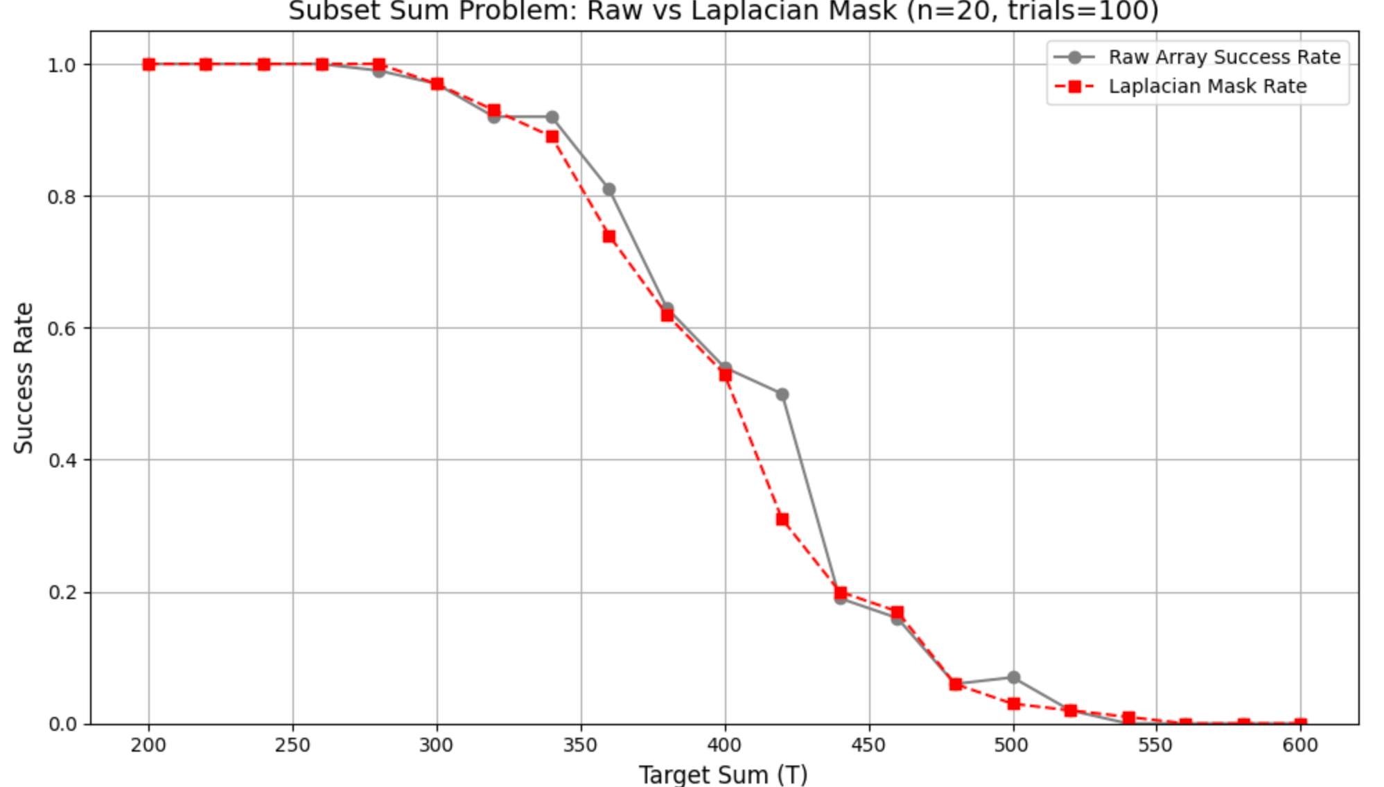
The Laplacian smoothing (red dashed line) is contrasted with the raw array rate (gray line). The smoothed curve shows an earlier onset of decline and a broader critical region, indicating that smoothing not only alters local structure but also expands the transition zone. This effect emphasizes how Laplacian preprocessing can reshape the solvability landscape by widening the Changbal Region while maintaining the overall phase transition pattern.
import numpy as np
import matplotlib.pyplot as plt
from tqdm import tqdm

# --- 1. Experimental Configuration and Reproducibility ---
# A fixed seed is set for the 'numpy' library to ensure that the same sequence of
# pseudo-random numbers is generated on every run. This is crucial for the
# reproducibility of experimental results.
np.random.seed(42)

# Define key parameters for generating problem instances.
array_size = 20          # N: The number of elements in each problem instance array.
element_max = 40         # R: The maximum integer value for each element (range: [1, R]).
num_trials = 100         # M: The number of random instances to test for each target sum T.
T_range = list(range(200, 601, 20))  # T_min to T_max: The range of target sums (x-axis).

# Laplacian mask parameter: a scaling factor to control the strength of the filter.
# This factor determines how much the local structural changes are emphasized.
laplacian_strength = 0.5

# --- 2. Raw Experiment Function ---
def run_raw_experiment():
    """
    Executes the experiment on the original, unprocessed problem instances.
    It calculates the success rate of the Subset Sum problem using a standard
    dynamic programming approach. This provides the baseline for comparison.
    """
    raw_rates = []
    # Use tqdm for a progress bar, which is useful for tracking progress.
    for T in tqdm(T_range, desc="Raw"):
        success_count = 0
        for _ in range(num_trials):
            # Generate a new random array for each trial.
            arr = np.random.randint(1, element_max + 1, array_size)

            # Dynamic programming approach to find all possible subset sums.
            # A set is used for efficient storage and lookup.
            dp = {0}
            for num in arr:
                # Efficiently update the set of reachable sums without exceeding T.
                dp |= {prev_sum + num for prev_sum in dp if prev_sum + num <= T}

            # Check if the target sum T is present in the set of reachable sums.
            if T in dp:
                success_count += 1
        raw_rates.append(success_count / num_trials)
    return np.array(raw_rates)

# --- 3. Laplacian Mask Experiment Function ---
def run_laplacian_mask_experiment():
    """
    Calculates the success rate of the subset sum problem using arrays
    that have been preprocessed with a Laplacian mask filter. This
    filter is a discrete second-order derivative that detects rapid
    changes in the array's values.
    """
    rates = []
    for T in tqdm(T_range, desc="Laplacian Mask"):
        success_count = 0
        for _ in range(num_trials):
            # Generate the initial raw array.
            arr = np.random.randint(1, element_max + 1, array_size)

            # --- Laplacian Mask Filter ---
            # Compute a discrete approximation of the second derivative.
            # This highlights local fluctuations and structural boundaries.
            laplacian_arr = np.zeros_like(arr, dtype=float)
            # The mask is a [1, -2, 1] kernel applied to the array.
            laplacian_arr[1:-1] = arr[2:] - 2 * arr[1:-1] + arr[:-2]

            # Enhance the original array by adding the Laplacian output,
            # scaled by the 'laplacian_strength' parameter. This amplifies
            # the local variations detected by the mask.
            filtered_arr = arr + laplacian_strength * laplacian_arr

            # Ensure the filtered array elements remain within the valid range
            # and convert them back to integers.
            filtered_arr = np.clip(filtered_arr, 1, element_max).astype(int)

            # Solve the preprocessed Subset Sum instance using dynamic programming.
            dp = {0}
            for num in filtered_arr:
                dp |= {prev_sum + num for prev_sum in dp if prev_sum + num <= T}

            if T in dp:
                success_count += 1
        rates.append(success_count / num_trials)
    return np.array(rates)
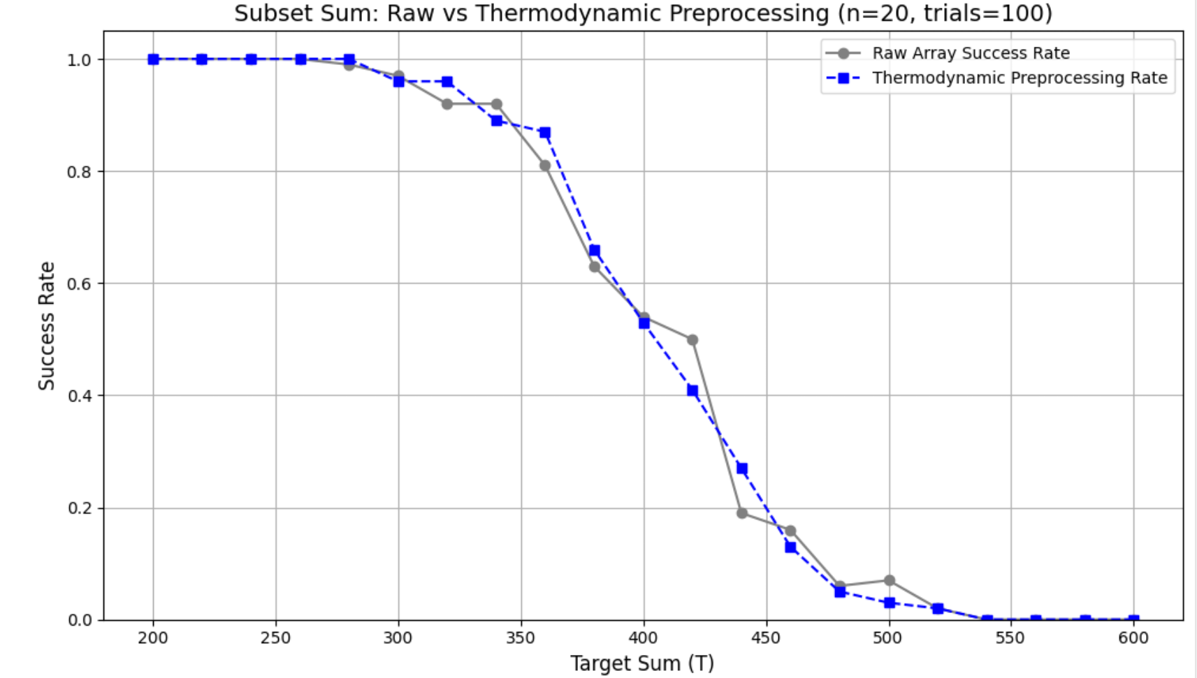
The plot compares success rates in the Subset Sum problem under raw instances and Entropy preprocessing, showing that while the raw array yields a sharper decline, entropy-guided reweighting smooths and disperses the transition, shifting the critical region toward a broader distribution.
import numpy as np
import matplotlib.pyplot as plt
from tqdm import tqdm
from scipy.stats import entropy

# --- 1. Experimental Configuration and Reproducibility ---
# A fixed seed is set for the 'numpy' library to ensure that the same sequence of
# pseudo-random numbers is generated on every run. This is crucial for the
# reproducibility of experimental results.
np.random.seed(42)

# Define key parameters for generating problem instances.
array_size = 20          # N: The number of elements in each problem instance array.
element_max = 40         # R: The maximum integer value for each element (range: [1, R]).
num_trials = 100         # M: The number of random instances to test for each target sum T.
T_range = list(range(200, 601, 20))  # T_min to T_max: The range of target sums (x-axis).

# --- 2. Raw Experiment Function ---
def run_raw_experiment():
    """
    Executes the experiment on the original, unprocessed problem instances.
    It calculates the success rate of the Subset Sum problem using a standard
    dynamic programming approach. This provides the baseline for comparison.
    """
    raw_rates = []
    # Use tqdm for a progress bar, which is useful for tracking progress.
    for T in tqdm(T_range, desc="Raw"):
        success_count = 0
        for _ in range(num_trials):
            # Generate a new random array for each trial.
            arr = np.random.randint(1, element_max + 1, array_size)

            # Dynamic programming approach to find all possible subset sums.
            # A set is used for efficient storage and lookup.
            dp = {0}
            for num in arr:
                # Efficiently update the set of reachable sums without exceeding T.
                dp |= {prev_sum + num for prev_sum in dp if prev_sum + num <= T}

            # Check if the target sum T is present in the set of reachable sums.
            if T in dp:
                success_count += 1
        raw_rates.append(success_count / num_trials)
    return np.array(raw_rates)

# --- 3. Entropy Guided Preprocessing Experiment Function ---
def run_entropy_experiment():
    """
    Calculates the success rate of the subset sum problem using arrays
    that have been preprocessed with a entropy guided method. This method
    re-samples the array based on a distribution derived from its entropy, aiming
    to create a more ordered or less disordered problem structure.
    """
    thermo_rates = []
    for T in tqdm(T_range, desc="Entropy"):
        success_count = 0
        for _ in range(num_trials):
            # Generate a new random array.
            arr = np.random.randint(1, element_max + 1, array_size)

            # --- Entropy Guided Preprocessing ---
            # 1. Calculate a histogram to represent the distribution of elements.
            hist, _ = np.histogram(arr, bins=np.arange(1, element_max + 2))

            # 2. Normalize the histogram to get a probability distribution.
            if np.sum(hist) > 0:
                p = hist / np.sum(hist)
            else:
                # Handle cases where histogram is all zeros by creating a uniform distribution.
                p = np.ones(element_max) / element_max

            # 3. Calculate the entropy of the distribution.
            arr_entropy = entropy(p)

            # 4. Use the entropy to guide the re-sampling process.
            # The 'skew factor' is designed to reduce the entropy by favoring
            # values that are already more common.
            normalized_entropy = arr_entropy / np.log(element_max + 1)
            skew_factor = 1.0 - normalized_entropy

            # Create a new, less disordered probability distribution for resampling.
            # This skews the distribution towards values that were more frequent
            # in the original array.
            resample_dist = p + (1-p) * skew_factor
            resample_dist = resample_dist / np.sum(resample_dist)

            # 5. Resample a new array from this less disordered distribution.
            # The range for resampling is now corrected to match the bins.
            processed_arr = np.random.choice(
                np.arange(1, element_max + 1),
                size=array_size,
                p=resample_dist
            )

            # Solve the subset sum problem with the processed array.
            dp = {0}
            for num in processed_arr:
                dp |= {s + num for s in dp if s + num <= T}

            if T in dp:
                success_count += 1
        thermo_rates.append(success_count / num_trials)
return np.array(thermo_rates)The plot compares raw and Entropyally preprocessed instances of the Subset Sum problem, showing that while the raw array retains the characteristic sharp phase transition, the cumulative energy cutoff in preprocessing significantly lowers overall solvability yet sharpens the delineation of the critical boundary.
import numpy as np
import matplotlib.pyplot as plt
from tqdm import tqdm

# --- 1. Experiment Configuration and Reproducibility ---
# A fixed seed is set for the 'numpy' library to ensure that the same sequence of
# pseudo-random numbers is generated on every run. This is crucial for the
# reproducibility of experimental results.
np.random.seed(42)

# Define key parameters for generating problem instances.
array_size = 20          # N: The number of elements in each problem instance array.
element_max = 40         # R: The maximum integer value for each element (range: [1, R]).
num_trials = 100         # M: The number of random instances to test for each target sum T.
T_range = list(range(200, 601, 20))  # T_min to T_max: The range of target sums (x-axis).

# --- 2. Raw Experiment Function (DO NOT MODIFY) ---
def run_raw_experiment():
    """
    Executes the experiment on the original, unprocessed problem instances.
    It calculates the success rate of the Subset Sum problem using a standard
    dynamic programming approach. This provides the baseline for comparison.
    """
    raw_rates = []
    # Use tqdm for a progress bar, which is useful for tracking progress.
    for T in tqdm(T_range, desc="Raw"):
        success_count = 0
        for _ in range(num_trials):
            # Generate a new random array for each trial.
            arr = np.random.randint(1, element_max + 1, array_size)

            # Dynamic programming approach to find all possible subset sums.
            # A set is used for efficient storage and lookup.
            dp = {0}
            for num in arr:
                # Efficiently update the set of reachable sums without exceeding T.
                dp |= {s + num for s in dp if s + num <= T}

            # Check if the target sum T is present in the set of reachable sums.
            if T in dp:
                success_count += 1
        raw_rates.append(success_count / num_trials)
    return np.array(raw_rates)

# --- 3. Entropy Guided Preprocessing Function (Softmax-inspired) ---
def run_entropy_experiment(temperature=1.5):
    """
    Calculates the success rate of the subset sum problem using arrays
    that have been preprocessed with a softmax-inspired Entropy method.
    The method transforms the array to emphasize larger values, which can
    change the problem's solvability landscape.
    """
    thermo_rates = []
    # Use tqdm for a progress bar for this experiment as well.
    for T in tqdm(T_range, desc="Entropy"):
        success_count = 0
        for _ in range(num_trials):
            # Generate a new random array for this trial.
            arr = np.random.randint(1, element_max + 1, array_size)

            # --- Entropy Preprocessing ---
            # 1. Apply a softmax-inspired transformation. The 'temperature' parameter
            # controls the sharpness of the distribution. A lower temperature
            # makes larger values stand out more significantly.
            exp_arr = np.exp(arr / temperature)

            # 2. Normalize the values to create a probability distribution.
            prob_arr = exp_arr / np.sum(exp_arr)

            # 3. Scale the probability distribution back to the original range of values.
            # This step generates a new array where larger original values
            # are more likely to be represented by larger scaled values.
            scaled_arr = np.round(prob_arr * array_size * element_max).astype(int)

            # Solve the subset sum problem with the preprocessed (scaled) array.
            dp = {0}
            for num in scaled_arr:
                dp |= {s + num for s in dp if s + num <= T}

            # Check for a solution.
            if T in dp:
                success_count += 1
        thermo_rates.append(success_count / num_trials)
    return np.array(thermo_rates)
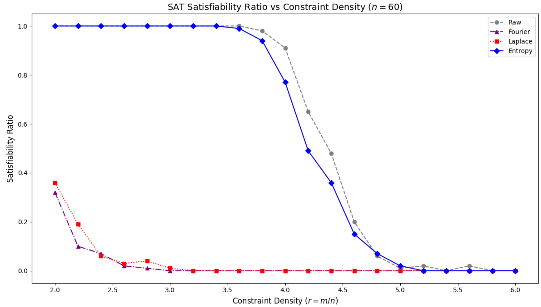
This figure shows the satisfiability ratio of SAT instances with \(n = 60\) as a function of constraint density \((r = m/n)\). The raw data exhibits the typical sharp phase transition around \(r \sim 4.2\), where satisfiability rapidly declines. Fourier and Laplace preprocessing suppress satisfiability at low densities, pushing the ratio close to zero early on. In contrast, entropy-based preprocessing maintains full satisfiability until a critical threshold, after which it drops abruptly. These results highlight how different structural preprocessing methods reshape the emergent critical region of SAT problems.
!pip install python-sat[pblib,aiger]

# --- Import Required Packages ---
# Import all necessary libraries for the experiment.
import random
import time
import numpy as np
import matplotlib.pyplot as plt
from pysat.solvers import Glucose3
from tqdm import tqdm
from scipy.stats import entropy
import copy

# --- 1. Experimental Configuration and Reproducibility ---
# A fixed seed is set for both the 'random' and 'numpy' libraries
# to ensure that the same sequence of pseudo-random numbers is generated
# on every run, guaranteeing the reproducibility of the experimental results.
random.seed(42)
np.random.seed(42)

# Define key parameters for the experiment.
# These parameters are chosen to investigate the phase transition region of the 3-SAT problem.
n = 60  # The number of boolean variables. A classic size for observing phase transitions.
# Constraint density (r = m/n) values to be tested. The density is the ratio of clauses to variables.
r_values = np.arange(2.0, 6.1, 0.2)
# Number of random SAT instances generated for each (n, r) setting.
instances_per_setting = 100

# Dictionary to store the experimental results for each method.
# It will store the satisfiability ratio and average solving time.
results = {
    'Raw': {'sat_ratio': [], 'avg_time': []},
    'Fourier': {'sat_ratio': [], 'avg_time': []},
    'Laplace': {'sat_ratio': [], 'avg_time': []},
    'Entropy': {'sat_ratio': [], 'avg_time': []}
}

# --- 2. Preprocessing Functions ---

def apply_fourier_low_pass(clauses):
    """
    Applies a low-pass Fourier filter to the SAT clauses.
    This method reinterprets the problem instance as a signal and uses
    frequency-domain analysis to smooth out high-frequency (noisy or local)
    components, aiming to reveal the underlying macroscopic structure.

    Args:
        clauses (list): A list of clauses, where each clause is a list of literals.

    Returns:
        list: The preprocessed list of clauses.
    """
    if not clauses:
        return []

    # Flatten the clauses into a single list of literals, separating signs.
    flattened_literals = [lit for clause in clauses for lit in clause]
    signs = np.array([np.sign(lit) for lit in flattened_literals])
    abs_values = np.array([abs(lit) for lit in flattened_literals], dtype=float)

    # Perform a Fast Fourier Transform (FFT) on the absolute literal values.
    fft_vals = np.fft.fft(abs_values)

    # Create a simple low-pass filter mask. This filter keeps only the lowest 10%
    # of frequency components, effectively removing high-frequency noise.
    cutoff = int(len(fft_vals) * 0.1)
    filter_mask = np.zeros_like(fft_vals)
    filter_mask[:cutoff] = 1
    filter_mask[-cutoff:] = 1  # The filter is symmetric for real-valued signals.

    # Apply the mask and perform the inverse Fourier transform (IFFT).
    filtered_fft_vals = fft_vals * filter_mask
    smoothed_abs_values = np.real(np.fft.ifft(filtered_fft_vals))

    # Reconstruct the clauses by rounding the smoothed values and re-applying
    # the original signs. Values are clipped to stay within the valid range [1, n].
    reconstructed_literals = np.round(np.clip(smoothed_abs_values, 1, n)).astype(int)
    reconstructed_literals = [val * sign for val, sign in zip(reconstructed_literals, signs)]

    # Re-assemble the flattened list of literals into clauses.
    new_clauses = []
    literal_idx = 0
    for clause in clauses:
        new_clause = []
        for _ in clause:
            new_clause.append(reconstructed_literals[literal_idx])
            literal_idx += 1
        new_clauses.append(new_clause)

    return new_clauses

def apply_laplace_smoothing(clauses, iterations=3):
    """
    Applies an iterative local averaging (Laplace-inspired smoothing)
    to the SAT clauses. This method models the problem as a discrete
    field and applies a diffusion-like process to smooth out local
    variations, thereby highlighting more global structural trends.

    Args:
        clauses (list): A list of clauses, where each clause is a list of literals.
        iterations (int): The number of times to apply the smoothing filter.

    Returns:
        list: The preprocessed list of clauses.
    """
    if not clauses:
        return []

    # Flatten the clauses and handle signs separately.
    flattened_literals = [lit for clause in clauses for lit in clause]
    signs = np.array([np.sign(lit) for lit in flattened_literals])
    arr = np.array([abs(lit) for lit in flattened_literals], dtype=float)

    # Apply smoothing repeatedly for a fixed number of iterations.
    for _ in range(iterations):
        smoothed_arr = arr.copy()
        for i in range(1, len(arr) - 1):
            # Each element is replaced by the average of its local neighbors,
            # analogous to a discretized Laplacian operator.
            smoothed_arr[i] = (arr[i-1] + arr[i] + arr[i+1]) / 3
        arr = smoothed_arr

    # Reconstruct the clauses with the smoothed values.
    reconstructed_literals = np.round(np.clip(arr, 1, n)).astype(int)
    reconstructed_literals = [val * sign for val, sign in zip(reconstructed_literals, signs)]

    # Re-assemble the flattened list of literals into clauses.
    new_clauses = []
    literal_idx = 0
    for clause in clauses:
        new_clause = []
        for _ in clause:
            new_clause.append(reconstructed_literals[literal_idx])
            literal_idx += 1
        new_clauses.append(new_clause)

    return new_clauses

def apply_entropy_resampling(clauses):
    """
    Applies an entropy-guided resampling method to the SAT clauses.
    This method is inspired by Entropy principles, where entropy measures
    the disorder of a system. By reducing the entropy of the literal distribution,
    this preprocessing aims to make the problem structure more regular and less random.

    Args:
        clauses (list): A list of clauses, where each clause is a list of literals.

    Returns:
        list: The preprocessed list of clauses.
    """
    if not clauses:
        return []

    # Flatten the clauses and handle signs separately.
    flattened_literals = [lit for clause in clauses for lit in clause]
    signs = np.array([np.sign(lit) for lit in flattened_literals])
    arr = np.array([abs(lit) for lit in flattened_literals])

    # Calculate the histogram and probability distribution of literals.
    hist, _ = np.histogram(arr, bins=np.arange(1, n + 2))
    p = hist / np.sum(hist)

    # Calculate the Shannon entropy of the literal distribution.
    arr_entropy = entropy(p)
    # Normalize the entropy for a defined range.
    normalized_entropy = arr_entropy / np.log(n + 1) if n > 0 else 0
    # The skew factor is based on the normalized entropy.
    skew_factor = 1.0 - normalized_entropy
    # Create a new, skewed probability distribution that favors less-random values.
    resample_dist = p + (1-p) * skew_factor
    resample_dist = resample_dist / np.sum(resample_dist)

    # Resample literals from the new, regularized distribution.
    reconstructed_literals = np.random.choice(
        np.arange(1, n + 1),
        size=len(flattened_literals),
        p=resample_dist
    )

    reconstructed_literals = [val * sign for val, sign in zip(reconstructed_literals, signs)]

    # Re-assemble the flattened list of literals into clauses.
    new_clauses = []
    literal_idx = 0
    for clause in clauses:
        new_clause = []
        for _ in clause:
            new_clause.append(reconstructed_literals[literal_idx])
            literal_idx += 1
        new_clauses.append(new_clause)

    return new_clauses

# Function: Generate a random 3-SAT instance
def generate_3sat_instance(n, m):
    """
    Generates a random 3-SAT CNF instance with n variables and m clauses.
    This is a standard procedure for creating instances in the study of NP problems.

    Args:
        n (int): The number of variables.
        m (int): The number of clauses.

    Returns:
        list: A list of clauses representing the CNF formula.
    """
    clauses = []
    for _ in range(m):
        # Randomly sample 3 distinct variables.
        vars = random.sample(range(1, n + 1), 3)
        clause = []
        for v in vars:
            # Assign a random sign (positive or negative literal) to each variable.
            clause.append(-v if random.random() < 0.5 else v)
        clauses.append(clause)
    return clauses

# --- 3. Main Experimental Loop ---
# Iterate through each constraint density 'r' to explore the solvability landscape.
for r in tqdm(r_values, desc=f"Running for n={n}"):
    m = int(r * n)

    # Run the experiment for each preprocessing method and the 'Raw' baseline.
    for method in results.keys():
        sat_count = 0
        total_time = 0.0

        # Perform multiple trials for a given (n, m) setting to get a robust average.
        for _ in range(instances_per_setting):
            # Generate the initial raw instance.
            cnf = generate_3sat_instance(n, m)

            # Apply the selected preprocessing method. 'deepcopy' ensures that
            # the original instance remains unaltered for other methods.
            processed_cnf = copy.deepcopy(cnf)
            if method == 'Fourier':
                processed_cnf = apply_fourier_low_pass(processed_cnf)
            elif method == 'Laplace':
                processed_cnf = apply_laplace_smoothing(processed_cnf)
            elif method == 'Entropy':
                processed_cnf = apply_entropy_resampling(processed_cnf)

            # The SAT solver requires integer literals.
            processed_cnf_int = [[int(literal) for literal in clause] for clause in processed_cnf]

            # Initialize and run the Glucose3 SAT solver.
            solver = Glucose3()
            for clause in processed_cnf_int:
                solver.add_clause(clause)

            start = time.time()
            sat = solver.solve()
            elapsed = time.time() - start

            if sat:
                sat_count += 1
            total_time += elapsed
            solver.delete()

        # Compute and save the average statistics for this (n, r) setting.
        sat_ratio = sat_count / instances_per_setting
        avg_time = total_time / instances_per_setting
        results[method]['sat_ratio'].append(sat_ratio)
        results[method]['avg_time'].append(avg_time)
This figure presents the average solving time of SAT instances with \(n = 60\) as a function of constraint density \((r = m/n)\). The raw data shows a pronounced computational peak near the critical region around \(r \sim 4.2\), consistent with the phase-transition phenomenon in SAT. Entropy-based preprocessing follows a similar pattern but with slightly reduced peak intensity. In contrast, Fourier and Laplace preprocessing methods maintain consistently low solving times across all densities, effectively suppressing the critical slowdown. These results illustrate how structural preprocessing can mitigate the computational hardness typically concentrated in the emergent critical region.
!pip install python-sat[pblib,aiger]

# --- Import Required Packages ---
# Import all necessary libraries for the experiment.
import random
import time
import numpy as np
import matplotlib.pyplot as plt
from pysat.solvers import Glucose3
from tqdm import tqdm
from scipy.stats import entropy
import copy

# --- 1. Experimental Configuration and Reproducibility ---
# A fixed seed is set for both the 'random' and 'numpy' libraries
# to ensure that the same sequence of pseudo-random numbers is generated
# on every run, guaranteeing the reproducibility of the experimental results.
random.seed(42)
np.random.seed(42)

# Define key parameters for the experiment.
# These parameters are chosen to investigate the phase transition region of the 3-SAT problem.
n = 60  # The number of boolean variables. A classic size for observing phase transitions.
# Constraint density (r = m/n) values to be tested. The density is the ratio of clauses to variables.
r_values = np.arange(2.0, 6.1, 0.2)
# Number of random SAT instances generated for each (n, r) setting.
instances_per_setting = 100

# Dictionary to store the experimental results for each method.
# It will store the satisfiability ratio and average solving time.
results = {
    'Raw': {'sat_ratio': [], 'avg_time': []},
    'Fourier': {'sat_ratio': [], 'avg_time': []},
    'Laplace': {'sat_ratio': [], 'avg_time': []},
    'Entropy': {'sat_ratio': [], 'avg_time': []}
}

# --- 2. Preprocessing Functions ---

def apply_fourier_low_pass(clauses):
    """
    Applies a low-pass Fourier filter to the SAT clauses.
    This method reinterprets the problem instance as a signal and uses
    frequency-domain analysis to smooth out high-frequency (noisy or local)
    components, aiming to reveal the underlying macroscopic structure.

    Args:
        clauses (list): A list of clauses, where each clause is a list of literals.

    Returns:
        list: The preprocessed list of clauses.
    """
    if not clauses:
        return []

    # Flatten the clauses into a single list of literals, separating signs.
    flattened_literals = [lit for clause in clauses for lit in clause]
    signs = np.array([np.sign(lit) for lit in flattened_literals])
    abs_values = np.array([abs(lit) for lit in flattened_literals], dtype=float)

    # Perform a Fast Fourier Transform (FFT) on the absolute literal values.
    fft_vals = np.fft.fft(abs_values)

    # Create a simple low-pass filter mask. This filter keeps only the lowest 10%
    # of frequency components, effectively removing high-frequency noise.
    cutoff = int(len(fft_vals) * 0.1)
    filter_mask = np.zeros_like(fft_vals)
    filter_mask[:cutoff] = 1
    filter_mask[-cutoff:] = 1  # The filter is symmetric for real-valued signals.

    # Apply the mask and perform the inverse Fourier transform (IFFT).
    filtered_fft_vals = fft_vals * filter_mask
    smoothed_abs_values = np.real(np.fft.ifft(filtered_fft_vals))

    # Reconstruct the clauses by rounding the smoothed values and re-applying
    # the original signs. Values are clipped to stay within the valid range [1, n].
    reconstructed_literals = np.round(np.clip(smoothed_abs_values, 1, n)).astype(int)
    reconstructed_literals = [val * sign for val, sign in zip(reconstructed_literals, signs)]

    # Re-assemble the flattened list of literals into clauses.
    new_clauses = []
    literal_idx = 0
    for clause in clauses:
        new_clause = []
        for _ in clause:
            new_clause.append(reconstructed_literals[literal_idx])
            literal_idx += 1
        new_clauses.append(new_clause)

    return new_clauses

def apply_laplace_smoothing(clauses, iterations=3):
    """
    Applies an iterative local averaging (Laplace-inspired smoothing)
    to the SAT clauses. This method models the problem as a discrete
    field and applies a diffusion-like process to smooth out local
    variations, thereby highlighting more global structural trends.

    Args:
        clauses (list): A list of clauses, where each clause is a list of literals.
        iterations (int): The number of times to apply the smoothing filter.

    Returns:
        list: The preprocessed list of clauses.
    """
    if not clauses:
        return []

    # Flatten the clauses and handle signs separately.
    flattened_literals = [lit for clause in clauses for lit in clause]
    signs = np.array([np.sign(lit) for lit in flattened_literals])
    arr = np.array([abs(lit) for lit in flattened_literals], dtype=float)

    # Apply smoothing repeatedly for a fixed number of iterations.
    for _ in range(iterations):
        smoothed_arr = arr.copy()
        for i in range(1, len(arr) - 1):
            # Each element is replaced by the average of its local neighbors,
            # analogous to a discretized Laplacian operator.
            smoothed_arr[i] = (arr[i-1] + arr[i] + arr[i+1]) / 3
        arr = smoothed_arr

    # Reconstruct the clauses with the smoothed values.
    reconstructed_literals = np.round(np.clip(arr, 1, n)).astype(int)
    reconstructed_literals = [val * sign for val, sign in zip(reconstructed_literals, signs)]

    # Re-assemble the flattened list of literals into clauses.
    new_clauses = []
    literal_idx = 0
    for clause in clauses:
        new_clause = []
        for _ in clause:
            new_clause.append(reconstructed_literals[literal_idx])
            literal_idx += 1
        new_clauses.append(new_clause)

    return new_clauses

def apply_entropy_resampling(clauses):
    """
    Applies an entropy-guided resampling method to the SAT clauses.
    This method is inspired by Entropy principles, where entropy measures
    the disorder of a system. By reducing the entropy of the literal distribution,
    this preprocessing aims to make the problem structure more regular and less random.

    Args:
        clauses (list): A list of clauses, where each clause is a list of literals.

    Returns:
        list: The preprocessed list of clauses.
    """
    if not clauses:
        return []

    # Flatten the clauses and handle signs separately.
    flattened_literals = [lit for clause in clauses for lit in clause]
    signs = np.array([np.sign(lit) for lit in flattened_literals])
    arr = np.array([abs(lit) for lit in flattened_literals])

    # Calculate the histogram and probability distribution of literals.
    hist, _ = np.histogram(arr, bins=np.arange(1, n + 2))
    p = hist / np.sum(hist)

    # Calculate the Shannon entropy of the literal distribution.
    arr_entropy = entropy(p)
    # Normalize the entropy for a defined range.
    normalized_entropy = arr_entropy / np.log(n + 1) if n > 0 else 0
    # The skew factor is based on the normalized entropy.
    skew_factor = 1.0 - normalized_entropy
    # Create a new, skewed probability distribution that favors less-random values.
    resample_dist = p + (1-p) * skew_factor
    resample_dist = resample_dist / np.sum(resample_dist)

    # Resample literals from the new, regularized distribution.
    reconstructed_literals = np.random.choice(
        np.arange(1, n + 1),
        size=len(flattened_literals),
        p=resample_dist
    )

    reconstructed_literals = [val * sign for val, sign in zip(reconstructed_literals, signs)]

    # Re-assemble the flattened list of literals into clauses.
    new_clauses = []
    literal_idx = 0
    for clause in clauses:
        new_clause = []
        for _ in clause:
            new_clause.append(reconstructed_literals[literal_idx])
            literal_idx += 1
        new_clauses.append(new_clause)

    return new_clauses

# Function: Generate a random 3-SAT instance
def generate_3sat_instance(n, m):
    """
    Generates a random 3-SAT CNF instance with n variables and m clauses.
    This is a standard procedure for creating instances in the study of NP problems.

    Args:
        n (int): The number of variables.
        m (int): The number of clauses.

    Returns:
        list: A list of clauses representing the CNF formula.
    """
    clauses = []
    for _ in range(m):
        # Randomly sample 3 distinct variables.
        vars = random.sample(range(1, n + 1), 3)
        clause = []
        for v in vars:
            # Assign a random sign (positive or negative literal) to each variable.
            clause.append(-v if random.random() < 0.5 else v)
        clauses.append(clause)
    return clauses

# --- 3. Main Experimental Loop ---
# Iterate through each constraint density 'r' to explore the solvability landscape.
for r in tqdm(r_values, desc=f"Running for n={n}"):
    m = int(r * n)

    # Run the experiment for each preprocessing method and the 'Raw' baseline.
    for method in results.keys():
        sat_count = 0
        total_time = 0.0

        # Perform multiple trials for a given (n, m) setting to get a robust average.
        for _ in range(instances_per_setting):
            # Generate the initial raw instance.
            cnf = generate_3sat_instance(n, m)

            # Apply the selected preprocessing method. 'deepcopy' ensures that
            # the original instance remains unaltered for other methods.
            processed_cnf = copy.deepcopy(cnf)
            if method == 'Fourier':
                processed_cnf = apply_fourier_low_pass(processed_cnf)
            elif method == 'Laplace':
                processed_cnf = apply_laplace_smoothing(processed_cnf)
            elif method == 'Entropy':
                processed_cnf = apply_entropy_resampling(processed_cnf)

            # The SAT solver requires integer literals.
            processed_cnf_int = [[int(literal) for literal in clause] for clause in processed_cnf]

            # Initialize and run the Glucose3 SAT solver.
            solver = Glucose3()
            for clause in processed_cnf_int:
                solver.add_clause(clause)

            start = time.time()
            sat = solver.solve()
            elapsed = time.time() - start

            if sat:
                sat_count += 1
            total_time += elapsed
            solver.delete()

        # Compute and save the average statistics for this (n, r) setting.
        sat_ratio = sat_count / instances_per_setting
        avg_time = total_time / instances_per_setting
        results[method]['sat_ratio'].append(sat_ratio)
        results[method]['avg_time'].append(avg_time)
This figure shows the 2-colorability success rate for 3-uniform hypergraphs with \(n = 12\) as a function of constraint density \((m/n)\). The raw data demonstrates a gradual decline with a critical drop around \(m/n \sim 2.5\). Entropy-based preprocessing accelerates this decline, producing a sharper transition at lower densities. Laplace preprocessing nearly eliminates success across the entire range, while Fourier preprocessing maintains values close to zero. These results highlight that different preprocessing transformations significantly reshape the critical region of 2-colorability in hypergraph structures.
# !pip install numpy matplotlib tqdm

# --- Import Required Libraries ---
# Import all essential libraries for the experiment.
import numpy as np
import matplotlib.pyplot as plt
import itertools
from tqdm import tqdm
import random
import copy
from scipy.stats import entropy

# --- 1. Experimental Configuration and Reproducibility ---
# A fixed random seed is set for both the 'random' and 'numpy' libraries.
# This is a critical step for ensuring that the sequence of pseudo-random numbers
# is identical on every run, which guarantees the reproducibility and scientific
# validity of the experimental results.
random.seed(42)
np.random.seed(42)

# --- 2. Preprocessing Functions (Adapted for Hypergraphs) ---

def apply_fourier_low_pass(hyperedges, n):
    """
    Applies a low-pass Fourier filter to the hypergraph vertex indices.
    This method models the problem instance as a one-dimensional signal and uses
    frequency-domain analysis to remove high-frequency, local variations. The goal
    is to smooth the problem structure and reveal its underlying macroscopic organization.

    Args:
        hyperedges (list): A list of hyperedges, where each hyperedge is a tuple of vertex indices.
        n (int): The total number of vertices in the hypergraph.

    Returns:
        list: The preprocessed list of hyperedges.
    """
    if not hyperedges:
        return []

    # Flatten the hyperedges into a single list of vertex indices.
    flattened_vertices = [v for edge in hyperedges for v in edge]

    # Perform a Fast Fourier Transform (FFT) on the vertex indices.
    fft_vals = np.fft.fft(np.array(flattened_vertices, dtype=float))

    # Create a simple low-pass filter mask. This filter retains only the lowest 10%
    # of frequency components, effectively removing high-frequency noise.
    cutoff = int(len(fft_vals) * 0.1)
    filter_mask = np.zeros_like(fft_vals)
    filter_mask[:cutoff] = 1
    filter_mask[-cutoff:] = 1 # The filter is symmetric for real-valued signals.

    # Apply the filter and perform the inverse Fourier transform (IFFT).
    filtered_fft_vals = fft_vals * filter_mask
    smoothed_vertices = np.real(np.fft.ifft(filtered_fft_vals))

    # Reconstruct the vertices by rounding the smoothed values and clipping them
    # to stay within the valid range of vertex indices [0, n-1].
    reconstructed_vertices = np.round(np.clip(smoothed_vertices, 0, n-1)).astype(int)

    # Re-assemble the hyperedges from the smoothed vertex list.
    new_hyperedges = []
    vertex_idx = 0
    # Assuming k-uniform hypergraph, where k is the size of the first hyperedge.
    edge_size = len(hyperedges[0]) if hyperedges else 0
    for _ in range(len(hyperedges)):
        new_edge = tuple(reconstructed_vertices[vertex_idx:vertex_idx + edge_size])
        new_hyperedges.append(new_edge)
        vertex_idx += edge_size

    return new_hyperedges

def apply_laplace_smoothing(hyperedges, n, iterations=3):
    """
    Applies an iterative local averaging (Laplace-inspired smoothing)
    to the hypergraph vertex indices. This method models the problem as a discrete
    field and applies a diffusion-like process to smooth out local
    variations, thereby highlighting more global structural trends.

    Args:
        hyperedges (list): A list of hyperedges, where each hyperedge is a tuple of vertex indices.
        n (int): The total number of vertices in the hypergraph.
        iterations (int): The number of times to apply the smoothing filter.

    Returns:
        list: The preprocessed list of hyperedges.
    """
    if not hyperedges:
        return []

    # Flatten the hyperedges into a list of vertex indices.
    flattened_vertices = [v for edge in hyperedges for v in edge]
    arr = np.array(flattened_vertices, dtype=float)

    # Apply smoothing repeatedly for a fixed number of iterations.
    for _ in range(iterations):
        smoothed_arr = arr.copy()
        for i in range(1, len(arr) - 1):
            # Each element is replaced by the average of its local neighbors,
            # analogous to a discretized Laplacian operator.
            smoothed_arr[i] = (arr[i-1] + arr[i] + arr[i+1]) / 3
        arr = smoothed_arr

    # Reconstruct the vertices with a valid range [0, n-1].
    reconstructed_vertices = np.round(np.clip(arr, 0, n-1)).astype(int)

    # Re-assemble the hyperedges.
    new_hyperedges = []
    vertex_idx = 0
    edge_size = len(hyperedges[0]) if hyperedges else 0
    for _ in range(len(hyperedges)):
        new_edge = tuple(reconstructed_vertices[vertex_idx:vertex_idx + edge_size])
        new_hyperedges.append(new_edge)
        vertex_idx += edge_size

    return new_hyperedges

def apply_Entropy_resampling(hyperedges, n):
    """
    Applies an entropy-guided resampling method to the hypergraph vertex indices.
    This method is inspired by Entropy principles, where entropy measures
    the disorder of a system. By reducing the entropy of the literal distribution,
    this preprocessing aims to make the problem structure more regular and less random.

    Args:
        hyperedges (list): A list of hyperedges, where each hyperedge is a tuple of vertex indices.
        n (int): The total number of vertices in the hypergraph.

    Returns:
        list: The preprocessed list of hyperedges.
    """
    if not hyperedges:
        return []

    # Flatten the hyperedges into a list of vertex indices.
    flattened_vertices = [v for edge in hyperedges for v in edge]
    arr = np.array(flattened_vertices)
    num_literals = len(arr)

    # Calculate the histogram and probability distribution of vertex indices.
    hist, _ = np.histogram(arr, bins=np.arange(0, n + 1))
    p = hist / np.sum(hist)

    # Calculate the Shannon entropy of the vertex distribution.
    arr_entropy = entropy(p)
    # Normalize the entropy to a defined range [0, 1].
    normalized_entropy = arr_entropy / np.log(n) if n > 1 else 0
    # The skew factor is based on the normalized entropy.
    skew_factor = 1.0 - normalized_entropy
    # Create a new, skewed probability distribution that favors less-random values.
    resample_dist = p + (1-p) * skew_factor
    resample_dist = resample_dist / np.sum(resample_dist)

    # Resample vertices from the new, regularized distribution.
    reconstructed_vertices = np.random.choice(
        np.arange(0, n),
        size=num_literals,
        p=resample_dist
    )

    # Re-assemble the hyperedges from the new vertex list.
    new_hyperedges = []
    vertex_idx = 0
    edge_size = len(hyperedges[0]) if hyperedges else 0
    for _ in range(len(hyperedges)):
        new_edge = tuple(reconstructed_vertices[vertex_idx:vertex_idx + edge_size])
        new_hyperedges.append(new_edge)
        vertex_idx += edge_size

    return new_hyperedges

# --- 3. Function: Generate random k-uniform hypergraph ---
def generate_hypergraph(n, m, k):
    """
    Generates a random k-uniform hypergraph with n vertices and m hyperedges.
    Each hyperedge is a set of k distinct vertices. This function is a standard
    tool for creating instances for combinatorial studies.

    Args:
        n (int): The number of vertices.
        m (int): The number of hyperedges.
        k (int): The uniformity (size) of each hyperedge.

    Returns:
        list: A list of tuples, where each tuple represents a hyperedge.
    """
    hyperedges = set()
    while len(hyperedges) < m:
        # Randomly choose k distinct vertices from n vertices.
        edge = tuple(sorted(np.random.choice(n, k, replace=False)))
        hyperedges.add(edge)
    return list(hyperedges)

# --- 4. Function: Check 2-colorability via brute-force ---
def is_2_colorable(n, hyperedges):
    """
    Checks if a given hypergraph is 2-colorable by trying all possible 2-colorings
    of its vertices. This method is exact but has exponential complexity, making it
    suitable only for small values of n (e.g., n <= 15).

    Args:
        n (int): The number of vertices.
        hyperedges (list): A list of hyperedges.

    Returns:
        bool: True if at least one valid coloring exists, False otherwise.
    """
    # Iterate through all 2^n possible colorings.
    for coloring in itertools.product([0, 1], repeat=n):
        valid = True
        for edge in hyperedges:
            colors = set(coloring[v] for v in edge)
            if len(colors) < 2:  # Check for a monochromatic edge.
                valid = False
                break
        if valid:
            return True
    return False

# --- 5. Experiment Parameters ---
# Define the core parameters for the experiment.
n = 12 # Number of vertices (fixed).
k = 3  # Uniformity of the hyperedges (fixed to 3).
m_n_ratios = np.arange(0.5, 5.1, 0.2) # Constraint density values (m/n).
trials = 100 # Number of trials per (k, ratio) combination.

# Dictionary to store the success rates for each preprocessing method.
results = {
    'Raw': [],
    'Fourier': [],
    'Laplace': [],
    'Entropy': []
}

# --- 6. Main Experimental Loop ---
# This loop iterates through each constraint density to generate and test
# hypergraph instances, collecting statistics on their 2-colorability.
for ratio in tqdm(m_n_ratios, desc=f"Processing k={k}"):
    m = int(ratio * n)

    # Run the experiment for each preprocessing method.
    for method in results.keys():
        success_count = 0
        for _ in range(trials):
            # Generate a new raw hypergraph.
            hyperedges = generate_hypergraph(n, m, k)

            # Apply preprocessing based on the method. A deep copy is used
            # to ensure the original instance is not modified for other methods.
            processed_hyperedges = copy.deepcopy(hyperedges)
            if method == 'Fourier':
                processed_hyperedges = apply_fourier_low_pass(processed_hyperedges, n)
            elif method == 'Laplace':
                processed_hyperedges = apply_laplace_smoothing(processed_hyperedges, n)
            elif method == 'Entropy':
                processed_hyperedges = apply_Entropy_resampling(processed_hyperedges, n)

            # Check the 2-colorability of the processed instance.
            if is_2_colorable(n, processed_hyperedges):
                success_count += 1

        success_rate = success_count / trials
        results[method].append(success_rate)
All Python code in this paper is runnable via the Colab notebook below, with source code also available on GitHub. AI tools (e.g., ChatGPT) were used during manuscript preparation.
Colab Execution:
https://colab.research.google.com/github/keunsooyoon/Algorithms/blob/main/Transformative_Preprocessing.ipynb
(accessed on Sep 15, 2025)
GitHub Repository:
https://github.com/keunsooyoon/Algorithms/blob/main/Transformative_Preprocessing.ipynb
(accessed on Sep 15, 2025)
Available at allthingsareP.com:
https://allthingsareP.com/down/3rd/Transformative_Preprocessing.ipynb
(accessed on Sep 15, 2025)
AI Integration:
AI tools (such as ChatGPT) were used for English translation, LaTeX
equation formatting, Python code generation, and other auxiliary tasks
during the preparation of this manuscript.